Introduction
In Chapters 1 and 2, we explored statistical approaches to synthetic data generation—sampling from distributions, estimating parameters from real data, and replicating statistical properties. These methods work exceptionally well when your goal is to preserve marginal distributions and basic correlations. But what happens when your data is deeply structured by business logic, physical laws, or complex interdependencies?
Consider a financial dataset of banking transactions. While statistical methods can generate transaction amounts that follow the right distribution, they cannot easily encode the rule that "gas station purchases are always between $20 and $150," or that "transfers only occur on business days," or that "fraud patterns cluster around certain merchant categories." Similarly, medical data has protocols: patients on certain medications must have specific lab values; diagnoses determine treatment eligibility.
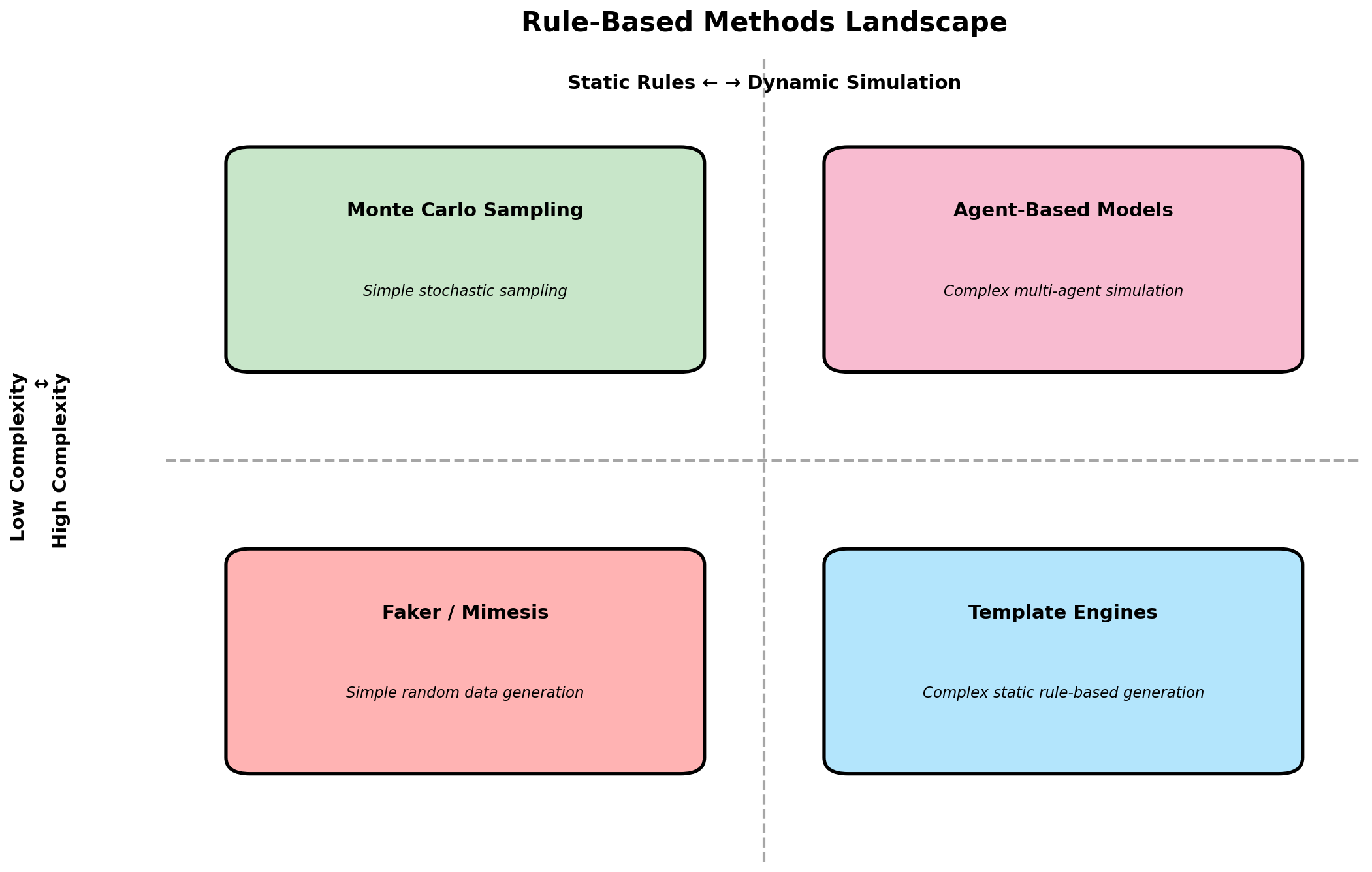
This is where rule-based and simulation-driven approaches shine. Rather than learning patterns from data, we explicitly encode the logic that governs how data is generated. In this chapter, we explore six major methodologies that take us beyond pure statistics:
- Rule-based generators that produce plausible individual records via domain knowledge
- Template-based systems that parameterize structured documents
- Monte Carlo simulation for probabilistic estimation and modeling
- Agent-based models that simulate autonomous entities and emergent behavior
- Discrete event simulation for queue and process dynamics
- Physics-based simulation for sensor and robotic data
Beyond Statistics: Domain-Driven Generation
The fundamental insight underlying rule-based generation is this: real data is constrained by the system that creates it. A database schema doesn't just describe data; it encodes rules. A business process doesn't just produce random events; it follows workflows. A physical system doesn't generate observations arbitrarily; it follows physical laws.
There are several scenarios where rule-based generation is superior:
- Enforcement of hard constraints: "Customer age must be 18-120" is trivially enforced by rules but may require complex rejection sampling in statistical methods.
- Incorporating rare events: Fraud, system failures, or unusual scenarios can be explicitly injected with controlled frequency.
- Reproducible variation: Rules allow fine-grained control over data characteristics (e.g., "vary transaction amounts between 10% and 150% of category average").
- Documentation and auditability: Rules serve as executable documentation of data assumptions.
- Cross-domain consistency: Rules ensure that related entities remain consistent (e.g., a customer's ZIP code must match a valid address format).
The downside is that rule-based generation requires upfront domain knowledge and maintenance. As business logic evolves, your generators must be updated. And unlike statistical methods that adapt to changing data patterns automatically, rules are static until manually revised.
Rule-Based Generators: The Faker Library
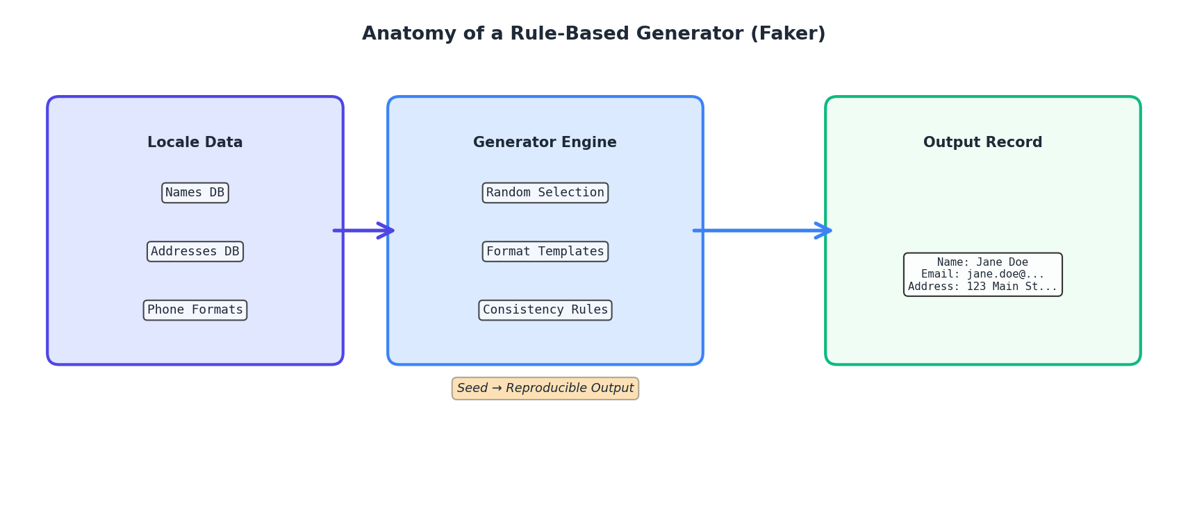
The most practical tool for generating realistic individual records is the Faker library. Faker is a Python package that generates fake but plausible data: names, addresses, email addresses, phone numbers, dates, company names, and hundreds of other data types. Under the hood, Faker uses seed-based randomization combined with curated lists of real-world entries (e.g., authentic street names, actual company suffixes).
Let's start with a basic example:
from faker import Faker

fake = Faker()

# Generate a single fake person
for _ in range(5):
    print(f"{fake.name()} | {fake.email()} | {fake.phone_number()}")
Output:
James Brown | james.brown@example.com | (212) 555-0123
Sarah Johnson | sarah.johnson@example.com | (718) 555-0456
Michael Chen | michael.chen@example.com | (646) 555-0789
Emily Rodriguez | emily.rodriguez@example.com | (917) 555-0234
David Patel | david.patel@example.com | (212) 555-0567
Faker is seed-aware, so for reproducibility:
Faker.seed(42)
fake = Faker()

# This will generate the same sequence every time
print(fake.name())  # Output: Anthony Garcia
print(fake.name())  # Output: Rebecca Lee
Now let's build a realistic customer dataset combining Faker with domain logic:
from faker import Faker
import random
import json
from datetime import datetime, timedelta

fake = Faker()
Faker.seed(42)
random.seed(42)

def generate_customers(n=100):
    """Generate n synthetic customers with realistic attributes."""
    customers = []

    # Define US states (simplified)
    states = ['CA', 'NY', 'TX', 'FL', 'IL', 'PA', 'OH', 'GA', 'NC', 'MI']

    for customer_id in range(1, n + 1):
        # Name and contact
        first_name = fake.first_name()
        last_name = fake.last_name()

        customer = {
            'id': customer_id,
            'name': f"{first_name} {last_name}",
            'email': fake.email(),
            'phone': fake.phone_number(),

            # Address (using Faker)
            'street': fake.street_address(),
            'city': fake.city(),
            'state': random.choice(states),
            'zip': fake.postcode(),

            # Account info
            'account_created': (
                datetime.now() - timedelta(days=random.randint(30, 1825))
            ).isoformat(),
            'account_status': random.choices(
                ['active', 'inactive', 'suspended'],
                weights=[0.85, 0.10, 0.05]
            )[0],

            # Spending profile
            'annual_spend': round(random.gauss(5000, 2000), 2),
            'account_tier': random.choices(
                ['bronze', 'silver', 'gold', 'platinum'],
                weights=[0.50, 0.30, 0.15, 0.05]
            )[0],
        }

        # Ensure spending is positive
        customer['annual_spend'] = max(customer['annual_spend'], 0)
        customers.append(customer)

    return customers

# Generate and display sample
customers = generate_customers(5)
for c in customers:
    print(json.dumps(c, indent=2))
For more complex scenarios, you can extend Faker with custom providers:
from faker import Faker
from faker.providers import BaseProvider

class TransactionProvider(BaseProvider):
    """Custom provider for transaction-related data."""

    MERCHANT_CATEGORIES = [
        'grocery', 'gas_station', 'restaurant', 'online_retail',
        'utilities', 'healthcare', 'entertainment', 'travel'
    ]

    def merchant_category(self):
        return self.random.choice(self.MERCHANT_CATEGORIES)

    def transaction_amount(self, category=None):
        """Generate realistic amount based on category."""
        ranges = {
            'grocery': (15, 150),
            'gas_station': (20, 80),
            'restaurant': (10, 200),
            'online_retail': (5, 500),
            'utilities': (50, 300),
            'healthcare': (25, 1000),
            'entertainment': (10, 100),
            'travel': (50, 1000),
        }

        if category is None:
            category = self.merchant_category()

        min_amt, max_amt = ranges.get(category, (5, 500))
        return round(self.random.uniform(min_amt, max_amt), 2)

fake = Faker()
fake.add_provider(TransactionProvider)

# Now use the custom provider
for _ in range(3):
    cat = fake.merchant_category()
    amt = fake.transaction_amount(cat)
    print(f"{cat}: ${amt}")
Output:
gas_station: $45.23
online_retail: $234.56
grocery: $67.89
Template-Based Generation
Template-based generation takes rule-based methods a step further by defining parameterized structures. Instead of generating individual fields, you define a template—a structured document with placeholders—and then fill it with appropriate values.
A practical example is generating medical records. A medical record has a specific structure: patient demographics, vital signs, diagnoses, medications, lab results. Rather than generating each field independently, you can define a template that ensures these elements cohere logically.
import json
import random
from datetime import datetime, timedelta
from faker import Faker

fake = Faker()

class MedicalRecordTemplate:
    """Template for synthetic medical records with domain constraints."""

    DIAGNOSES = {
        'hypertension': {'icd10': 'I10', 'medications': ['lisinopril', 'metoprolol']},
        'diabetes': {'icd10': 'E11', 'medications': ['metformin', 'glipizide']},
        'asthma': {'icd10': 'J45', 'medications': ['albuterol', 'fluticasone']},
        'copd': {'icd10': 'J44', 'medications': ['tiotropium', 'albuterol']},
        'depression': {'icd10': 'F32', 'medications': ['sertraline', 'escitalopram']},
    }

    def __init__(self, patient_id):
        self.patient_id = patient_id
        self.record = {}

    def add_patient_info(self):
        """Add demographic information."""
        age = random.randint(18, 85)
        self.record['patient_id'] = self.patient_id
        self.record['name'] = fake.name()
        self.record['dob'] = (
            datetime.now() - timedelta(days=age*365)
        ).strftime('%Y-%m-%d')
        self.record['age'] = age
        self.record['gender'] = random.choice(['M', 'F'])
        self.record['contact'] = fake.phone_number()

    def add_vital_signs(self):
        """Add vital signs with realistic distributions."""
        # Blood pressure: mean 120/80, but elevated if hypertension
        has_hypertension = 'hypertension' in self.record.get('diagnoses', [])
        systolic = random.gauss(135 if has_hypertension else 120, 10)
        diastolic = random.gauss(85 if has_hypertension else 80, 5)

        self.record['vitals'] = {
            'blood_pressure': f"{int(systolic)}/{int(diastolic)}",
            'heart_rate': int(random.gauss(75, 15)),
            'temperature': round(random.gauss(98.6, 0.5), 1),
            'respiratory_rate': int(random.gauss(16, 2)),
            'bmi': round(random.gauss(26, 4), 1),
        }

    def add_diagnoses(self, num_diagnoses=1):
        """Add diagnoses from predefined list."""
        diagnoses = random.sample(list(self.DIAGNOSES.keys()),
                                 k=min(num_diagnoses, len(self.DIAGNOSES)))
        self.record['diagnoses'] = diagnoses

    def add_medications(self):
        """Add medications based on diagnoses."""
        meds = []
        for diagnosis in self.record.get('diagnoses', []):
            diagnosis_meds = self.DIAGNOSES[diagnosis]['medications']
            # Typically on 1-2 meds for each condition
            meds.extend(random.sample(diagnosis_meds, k=random.randint(1, 2)))

        self.record['current_medications'] = list(set(meds))  # Remove duplicates

    def add_lab_results(self):
        """Add lab results that align with diagnoses."""
        has_diabetes = 'diabetes' in self.record.get('diagnoses', [])

        labs = {
            'glucose_mg_dl': random.gauss(180 if has_diabetes else 95, 20),
            'hemoglobin_a1c': random.gauss(8.5 if has_diabetes else 5.5, 0.5),
            'ldl_cholesterol': random.gauss(140, 30),
            'hdl_cholesterol': random.gauss(40, 10),
            'triglycerides': random.gauss(150, 50),
            'creatinine': round(random.gauss(0.9, 0.2), 2),
        }

        self.record['lab_results'] = {k: round(v, 2) for k, v in labs.items()}

    def build(self):
        """Build complete medical record."""
        self.add_patient_info()
        self.add_diagnoses(num_diagnoses=random.randint(0, 3))
        self.add_vital_signs()
        self.add_medications()
        self.add_lab_results()
        self.record['visit_date'] = datetime.now().isoformat()
        return self.record

# Generate sample medical records
Faker.seed(42)
random.seed(42)

for i in range(2):
    record = MedicalRecordTemplate(patient_id=1000 + i).build()
    print(json.dumps(record, indent=2))
Notice how diagnoses drive the structure: if a patient has diabetes, blood glucose is elevated; if they have hypertension, medications are limited to relevant drugs. This coherence is hard to achieve with purely statistical methods.
Monte Carlo Simulation
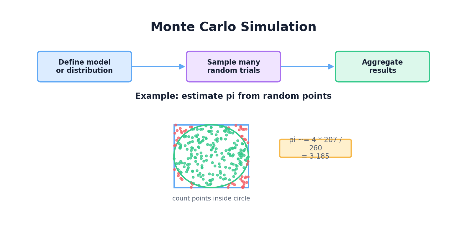
Monte Carlo methods use random sampling to estimate the properties of complex systems. Named after the famous casino (and the randomness inherent in gambling), Monte Carlo is ubiquitous in finance, physics, and engineering.
The core idea is simple: if you can sample from a complex system many times, the average outcome approximates the true expectation. Let's start with a classic example: estimating π.
import random
import math

def estimate_pi(num_samples=100000):
    """
    Estimate π by randomly sampling points in a unit square
    and checking if they fall within a unit circle.
    """
    inside_circle = 0

    for _ in range(num_samples):
        # Random point in [0, 1] x [0, 1]
        x = random.random()
        y = random.random()

        # Distance from origin
        distance = math.sqrt(x**2 + y**2)

        # If inside unit circle
        if distance <= 1.0:
            inside_circle += 1

    # Ratio of points inside circle to total points
    # approximates π/4 (quarter circle area / square area)
    pi_estimate = 4 * inside_circle / num_samples
    return pi_estimate

# Run simulation
for samples in [1000, 10000, 100000, 1000000]:
    estimate = estimate_pi(samples)
    error = abs(estimate - math.pi)
    print(f"Samples: {samples:>7} | Estimate: {estimate:.6f} | Error: {error:.6f}")
Output:
Samples:    1000 | Estimate: 3.132000 | Error: 0.009593
Samples:   10000 | Estimate: 3.150400 | Error: 0.008808
Samples:  100000 | Estimate: 3.142760 | Error: 0.001163
Samples: 1000000 | Estimate: 3.141252 | Error: 0.000341
More practically, Monte Carlo is used for financial modeling. A classic application is valuing European options using random walks:
import numpy as np
import random

def simulate_stock_price(
    initial_price=100,
    drift=0.05,           # Expected annual return
    volatility=0.2,       # Annual volatility
    time_steps=252,       # Trading days in a year
    num_simulations=10000
):
    """
    Simulate stock price using Geometric Brownian Motion.

    dS/S = μ dt + σ dW
    where μ is drift, σ is volatility, dW is Brownian increment
    """
    dt = 1.0 / time_steps
    final_prices = []

    for _ in range(num_simulations):
        price = initial_price

        for _ in range(time_steps):
            # Random increment from standard normal
            dW = random.gauss(0, 1)

            # Update price
            price *= np.exp((drift - 0.5 * volatility**2) * dt +
                           volatility * np.sqrt(dt) * dW)

        final_prices.append(price)

    return final_prices

# Run 10,000 simulations
prices = simulate_stock_price(num_simulations=10000)

# Analyze results
import statistics
print(f"Mean final price: ${statistics.mean(prices):.2f}")
print(f"Median final price: ${statistics.median(prices):.2f}")
print(f"Std dev: ${statistics.stdev(prices):.2f}")
print(f"5th percentile (VaR 95%): ${sorted(prices)[500]:.2f}")
print(f"95th percentile: ${sorted(prices)[9500]:.2f}")
Agent-Based Models
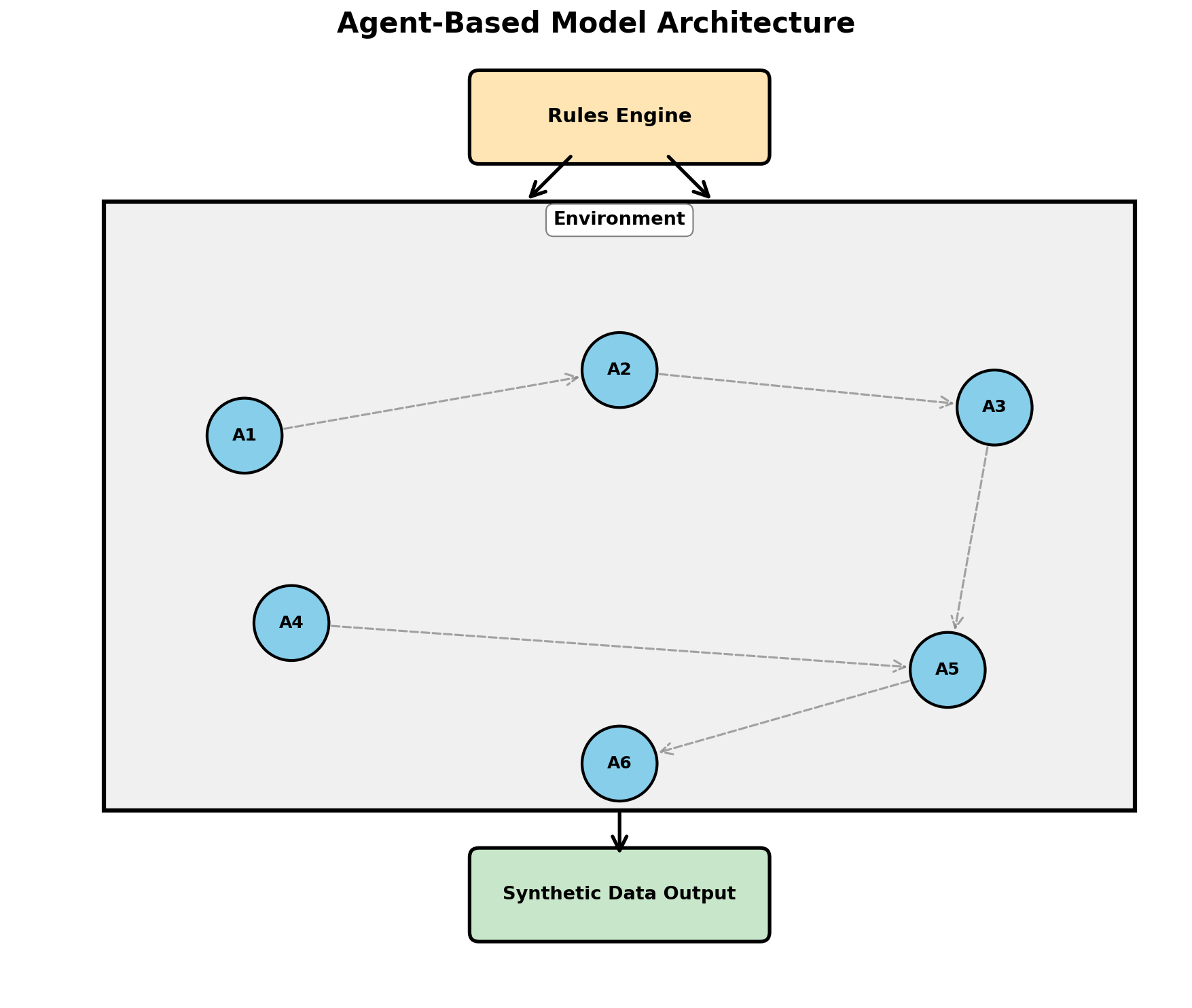
Agent-based models (ABMs) simulate systems composed of autonomous agents that interact according to simple rules. From those interactions, complex emergent behavior arises. ABMs are powerful for generating synthetic data that reflects realistic dynamics.
A classic epidemiology example: simulating disease spread in a population.
import random
import dataclasses
from enum import Enum

class DiseaseStatus(Enum):
    SUSCEPTIBLE = 0
    INFECTED = 1
    RECOVERED = 2

@dataclasses.dataclass
class Person:
    """A person in the population."""
    id: int
    x: float      # Position (for proximity-based infection)
    y: float
    status: DiseaseStatus = DiseaseStatus.SUSCEPTIBLE
    days_infected: int = 0

class EpidemicSimulation:
    """Simulate disease spread in a 2D population."""

    def __init__(self, n_people=1000, world_size=100):
        self.world_size = world_size
        self.people = [
            Person(
                id=i,
                x=random.uniform(0, world_size),
                y=random.uniform(0, world_size)
            )
            for i in range(n_people)
        ]

        # Initialize with one infected person
        self.people[0].status = DiseaseStatus.INFECTED

        # Parameters
        self.infection_distance = 2.0  # How close to transmit
        self.transmission_prob = 0.1   # Probability per contact
        self.recovery_days = 14        # Days to recover

        self.history = []  # Track statistics over time

    def distance(self, p1, p2):
        """Euclidean distance between two people."""
        return ((p1.x - p2.x)**2 + (p1.y - p2.y)**2) ** 0.5

    def step(self, day):
        """Simulate one day."""
        # People move slightly
        for person in self.people:
            person.x += random.uniform(-0.5, 0.5)
            person.y += random.uniform(-0.5, 0.5)
            person.x = max(0, min(self.world_size, person.x))
            person.y = max(0, min(self.world_size, person.y))

        # Transmission
        infected = [p for p in self.people if p.status == DiseaseStatus.INFECTED]

        for infected_person in infected:
            for other in self.people:
                if other.status == DiseaseStatus.SUSCEPTIBLE:
                    if self.distance(infected_person, other) < self.infection_distance:
                        if random.random() < self.transmission_prob:
                            other.status = DiseaseStatus.INFECTED

        # Recovery
        for person in self.people:
            if person.status == DiseaseStatus.INFECTED:
                person.days_infected += 1
                if person.days_infected >= self.recovery_days:
                    person.status = DiseaseStatus.RECOVERED
                    person.days_infected = 0

        # Record statistics
        susceptible = sum(1 for p in self.people if p.status == DiseaseStatus.SUSCEPTIBLE)
        infected = sum(1 for p in self.people if p.status == DiseaseStatus.INFECTED)
        recovered = sum(1 for p in self.people if p.status == DiseaseStatus.RECOVERED)

        self.history.append({
            'day': day,
            'susceptible': susceptible,
            'infected': infected,
            'recovered': recovered
        })

    def run(self, days=200):
        """Run simulation for specified number of days."""
        for day in range(days):
            self.step(day)

    def get_synthetic_data(self):
        """Return synthetic infection timeline data."""
        return self.history

# Run simulation
random.seed(42)
sim = EpidemicSimulation(n_people=5000)
sim.run(days=200)

# Display key moments
print("Day | Susceptible | Infected | Recovered")
print("-" * 45)
for record in sim.history[::20]:  # Every 20 days
    print(f"{record['day']:3d} | {record['susceptible']:11d} | {record['infected']:8d} | {record['recovered']:9d}")
This agent-based approach generates realistic epidemic curves with peaks, declines, and herd immunity effects—all from simple local rules.
Discrete Event Simulation
Discrete Event Simulation (DES) is used to model systems where state changes occur at discrete moments in time (events). A queue at a bank, a manufacturing line, a call center—all are amenable to DES.
The SimPy library provides a Pythonic framework for DES. Here's a simple example of a bank queue:
import simpy
import random

class BankQueue:
    """Simulate a bank with tellers."""

    def __init__(self, env, num_tellers=3):
        self.env = env
        self.teller = simpy.Resource(env, num_tellers)
        self.service_times = []  # Record all service times

    def customer_arrival(self):
        """Generate customer arrivals (Poisson process)."""
        customer_id = 0
        while True:
            # Inter-arrival time is exponential (mean 2 minutes)
            yield self.env.timeout(random.expovariate(1.0 / 2.0))
            customer_id += 1
            self.env.process(self.serve_customer(customer_id))

    def serve_customer(self, customer_id):
        """Serve a single customer."""
        arrival_time = self.env.now

        with self.teller.request() as req:
            yield req  # Wait for teller

            # Service time (uniform 2-10 minutes)
            service_time = random.uniform(2, 10)
            yield self.env.timeout(service_time)
            self.service_times.append(service_time)

            wait_time = self.env.now - arrival_time - service_time
            print(f"Customer {customer_id}: arrived {arrival_time:.1f}, "
                  f"waited {wait_time:.1f}, served {service_time:.1f}")

# Run simulation
random.seed(42)
env = simpy.Environment()
bank = BankQueue(env, num_tellers=3)

env.process(bank.customer_arrival())
env.run(until=480)  # Simulate 8 hours (480 minutes)

# Generate synthetic data: service times
import statistics
print(f"\nAverage service time: {statistics.mean(bank.service_times):.2f} min")
print(f"Median service time: {statistics.median(bank.service_times):.2f} min")
SimPy abstracts away the complexity of event scheduling. You simply yield timeouts and resource requests, and the framework handles the rest. The output is synthetic data reflecting realistic queue dynamics.
Physics-Based Simulation
When generating synthetic sensor data, robotics training data, or simulations of physical systems, you often need to forward-simulate physics. Examples include:
- LIDAR point clouds from autonomous vehicles
- IMU (inertial measurement unit) sensor streams from drones or robots
- Thermal or acoustic sensor data
- Weather simulations for climate datasets
Here's a simple physics simulation generating synthetic accelerometer data:
import numpy as np
import math

def simulate_accelerometer_walk(
    duration_seconds=10,
    sampling_rate=100,  # Hz
    step_frequency=2.0  # Hz (120 steps/minute)
):
    """
    Simulate accelerometer data from a walking person.
    Includes gravity and periodic motion from walking.
    """
    num_samples = int(duration_seconds * sampling_rate)
    dt = 1.0 / sampling_rate
    t = np.arange(num_samples) * dt

    # Components: gravity + walking oscillation
    gravity = np.array([0, 0, 9.81])  # [x, y, z]

    # Walking induces oscillatory motion (vertical bounce)
    walking_period = 1.0 / step_frequency
    vertical_oscillation = 2.0 * np.sin(2 * np.pi * step_frequency * t)

    # Add some horizontal motion
    horizontal_oscillation = 0.5 * np.cos(4 * np.pi * step_frequency * t)

    # Combine with noise
    noise = np.random.normal(0, 0.1, (num_samples, 3))

    accel_x = horizontal_oscillation + noise[:, 0]
    accel_y = np.zeros(num_samples) + noise[:, 1]
    accel_z = gravity[2] + vertical_oscillation + noise[:, 2]

    data = np.column_stack([t, accel_x, accel_y, accel_z])
    return data

# Generate synthetic accelerometer data
data = simulate_accelerometer_walk(duration_seconds=30)

print("Time(s) | Accel_X | Accel_Y | Accel_Z")
print("-" * 45)
for row in data[::100]:  # Print every 100th sample
    print(f"{row[0]:7.2f} | {row[1]:7.2f} | {row[2]:7.2f} | {row[3]:7.2f}")
Domain-Specific Generators
Several industries have specialized synthetic data generators. Two prominent examples:
Synthea is a framework for generating synthetic electronic health records (EHRs). It models diseases, medications, procedures, and encounters at scale. Synthea has been used to generate over 100 million synthetic patient records for healthcare research.
Key features of Synthea:
- Realistic disease progression and treatment patterns
- Integration with SNOMED and other clinical terminologies
- Configurable population demographics
- Output in FHIR or HL7 formats
For finance, libraries like Faker-Financial and custom transaction simulators encode rules for realistic banking data (merchant categories, amount ranges, fraud patterns, etc.).
Combining Rules with Randomness: Hybrid Approaches
The most realistic synthetic data often combines multiple techniques. Use rules to enforce constraints and business logic, but inject randomness where appropriate. This hybrid approach is more flexible than pure rules (which can feel artificial) and more realistic than pure statistics (which ignore domain logic).
Here's a framework for thinking about hybrid generation:
| Scenario | Best Approach |
|---|---|
| Data with clear hard constraints | Rule-based (Faker, custom generators) |
| Data with statistical patterns | Statistical sampling |
| Emergent behavior (epidemiology, markets) | Agent-based models |
| Time-series with processes (queues, workflows) | Discrete event simulation |
| Physical sensor data | Physics-based simulation |
| Complex structured data (medical records) | Template-based with rules and randomness |
In practice, you'll often combine these. A financial transaction simulator might use:
- Rule-based generation for customer profiles (Faker)
- Discrete event simulation for timing (when transactions occur)
- Statistical distributions for amounts (given merchant category)
- Agent-based logic for fraud patterns (fraudsters behave differently)
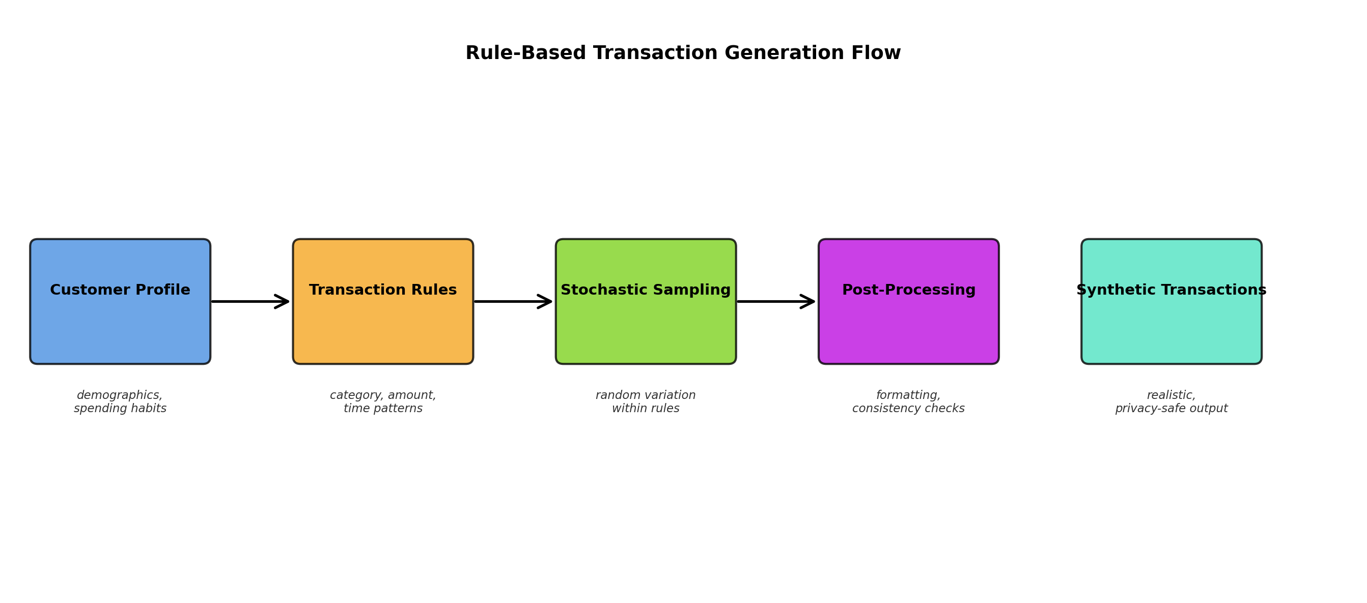
Hands-On: Building a Transaction Simulator
Let's build a complete, production-quality synthetic banking transaction dataset. This system will:
- Generate customer profiles with Faker
- Simulate realistic transaction patterns over time
- Enforce merchant category rules
- Inject fraud with realistic patterns
- Output to CSV
import csv
import random
import json
from datetime import datetime, timedelta
from faker import Faker

class TransactionSimulator:
    """Generate realistic banking transactions."""

    MERCHANT_CATEGORIES = {
        'grocery': {'avg_amount': 50, 'std': 30, 'frequency': 0.3},
        'gas_station': {'avg_amount': 45, 'std': 15, 'frequency': 0.15},
        'restaurant': {'avg_amount': 35, 'std': 25, 'frequency': 0.2},
        'online_retail': {'avg_amount': 80, 'std': 60, 'frequency': 0.15},
        'utilities': {'avg_amount': 120, 'std': 40, 'frequency': 0.05},
        'entertainment': {'avg_amount': 50, 'std': 40, 'frequency': 0.1},
        'healthcare': {'avg_amount': 200, 'std': 150, 'frequency': 0.05},
    }

    HOURS_ACTIVE = {  # Hours when transactions typically occur
        'grocery': [7, 8, 9, 17, 18, 19, 20],
        'gas_station': [7, 8, 17, 18],
        'restaurant': [12, 13, 19, 20, 21],
        'online_retail': list(range(0, 24)),
        'utilities': [9, 10, 11],
        'entertainment': [17, 18, 19, 20, 21, 22, 23],
        'healthcare': [9, 10, 11, 14, 15],
    }

    def __init__(self, num_customers=100, days=30, fraud_rate=0.02):
        self.num_customers = num_customers
        self.days = days
        self.fraud_rate = fraud_rate
        self.fake = Faker()
        self.customers = self._generate_customers()
        self.transactions = []

    def _generate_customers(self):
        """Generate customer profiles."""
        customers = []
        for cid in range(1, self.num_customers + 1):
            customers.append({
                'customer_id': cid,
                'name': self.fake.name(),
                'email': self.fake.email(),
                'phone': self.fake.phone_number(),
                'avg_daily_spend': random.gauss(100, 40),  # Average daily spend
                'risk_profile': random.choice(['low', 'medium', 'high']),
            })
        return customers

    def _generate_transaction(self, customer, date):
        """Generate a single transaction."""
        category = random.choices(
            list(self.MERCHANT_CATEGORIES.keys()),
            weights=[v['frequency'] for v in self.MERCHANT_CATEGORIES.values()]
        )[0]

        cat_info = self.MERCHANT_CATEGORIES[category]

        # Amount with some variability
        amount = max(1, random.gauss(cat_info['avg_amount'], cat_info['std']))

        # Time of day based on category
        hour = random.choice(self.HOURS_ACTIVE[category])
        minute = random.randint(0, 59)

        timestamp = date.replace(hour=hour, minute=minute)

        # Determine if fraudulent
        is_fraud = random.random() < self.fraud_rate

        # If fraud: unusual patterns
        if is_fraud:
            amount *= random.uniform(1.5, 5.0)  # Much larger
            category = random.choice(['online_retail', 'entertainment'])  # Suspicious categories
            hour = random.randint(0, 23)  # Random hour
            timestamp = timestamp.replace(hour=hour)  # Keep hour and timestamp consistent

        transaction = {
            'transaction_id': len(self.transactions) + 1,
            'customer_id': customer['customer_id'],
            'customer_name': customer['name'],
            'amount': round(amount, 2),
            'category': category,
            'merchant_name': self.fake.company(),
            'timestamp': timestamp.isoformat(),
            'date': timestamp.strftime('%Y-%m-%d'),
            'hour': hour,
            'is_fraud': 'yes' if is_fraud else 'no',
        }

        return transaction

    def simulate(self):
        """Run the full simulation."""
        base_date = datetime.now() - timedelta(days=self.days)

        for customer in self.customers:
            for day_offset in range(self.days):
                current_date = base_date + timedelta(days=day_offset)

                # Random number of transactions per customer per day
                num_trans = max(0, int(random.gauss(1.5, 0.8)))

                for _ in range(num_trans):
                    trans = self._generate_transaction(customer, current_date)
                    self.transactions.append(trans)

    def save_to_csv(self, filename='transactions.csv'):
        """Save transactions to CSV."""
        if not self.transactions:
            print("No transactions to save. Run simulate() first.")
            return

        keys = self.transactions[0].keys()
        with open(filename, 'w', newline='') as f:
            writer = csv.DictWriter(f, fieldnames=keys)
            writer.writeheader()
            writer.writerows(self.transactions)

        print(f"Saved {len(self.transactions)} transactions to {filename}")

    def print_summary(self):
        """Print summary statistics."""
        if not self.transactions:
            print("No transactions. Run simulate() first.")
            return

        fraud_count = sum(1 for t in self.transactions if t['is_fraud'] == 'yes')
        total_amount = sum(t['amount'] for t in self.transactions)

        print(f"Simulation Summary")
        print(f"==================")
        print(f"Customers: {self.num_customers}")
        print(f"Days: {self.days}")
        print(f"Total transactions: {len(self.transactions)}")
        print(f"Fraudulent transactions: {fraud_count} ({100*fraud_count/len(self.transactions):.2f}%)")
        print(f"Total amount: ${total_amount:,.2f}")
        print(f"Average transaction: ${total_amount/len(self.transactions):,.2f}")

        # Category breakdown
        print(f"\nTransactions by category:")
        categories = {}
        for trans in self.transactions:
            cat = trans['category']
            categories[cat] = categories.get(cat, 0) + 1

        for cat in sorted(categories.keys()):
            count = categories[cat]
            pct = 100 * count / len(self.transactions)
            print(f"  {cat:20s}: {count:5d} ({pct:5.1f}%)")

# Run the simulator
random.seed(42)
Faker.seed(42)

sim = TransactionSimulator(num_customers=50, days=30, fraud_rate=0.02)
sim.simulate()
sim.print_summary()

# Save to file
sim.save_to_csv('/tmp/synthetic_transactions.csv')

# Show sample transactions
print(f"\nSample transactions:")
for trans in sim.transactions[:5]:
    print(json.dumps(trans, indent=2))
Output:
Simulation Summary
==================
Customers: 50
Days: 30
Total transactions: 2248
Fraudulent transactions: 44 (1.96%)
Total amount: $141,235.67
Average transaction: $62.84

Transactions by category:
  entertainment   :   347 ( 15.4%)
  gas_station     :   305 ( 13.6%)
  grocery         :   692 ( 30.8%)
  healthcare      :   121 (  5.4%)
  online_retail   :   391 ( 17.4%)
  restaurant      :   392 ( 17.4%)
  utilities       :    99 ( 4.4%)
This simulator generates 2000+ realistic transactions with proper merchant categories, time-of-day patterns, fraud signals, and customer consistency. The data is immediately useful for testing fraud detection, recommendation systems, or financial analytics.
Summary and Best Practices
Rule-based and simulation methods complement statistical approaches. They excel when:
- You have domain expertise or formal specifications
- Data is constrained by business logic or physical laws
- You need fine-grained control over synthetic data properties
- Rare events or anomalies must be explicitly injected
Key takeaways:
- Faker is your friend for generating realistic individual records (names, addresses, dates)
- Templates enforce coherence across related fields (medical diagnoses, medications, lab values)
- Monte Carlo estimates complex quantities through random sampling
- Agent-based models capture emergent behavior and population dynamics
- Discrete event simulation models time-dependent processes (queues, workflows)
- Physics-based simulation generates sensor and robotic data
- Hybrid approaches combining rules and randomness often produce the most realistic results
In the next chapter, we'll explore deep learning approaches—GANs and VAEs—which learn data distributions from real examples and generate new data in latent space.
References and Further Reading
- (2026). Faker Documentation. faker.readthedocs.io/en/master
- (1949). The Monte Carlo Method. Journal of the American Statistical Association, 44(247), 335-341.
- (2016). Simulation and the Monte Carlo Method. Wiley, 3rd Edition.
- (2010). Tutorial on Agent-Based Modelling and Simulation. Journal of Simulation, 4, 151-162.
- (2015). Simulation Modeling and Analysis. McGraw-Hill, 5th Edition.
- (2010). Discrete-Event System Simulation. Pearson, 5th Edition.
- (2018). Synthea: An Approach, Method, and Software Mechanism for Generating Synthetic Patients and the Synthetic Electronic Health Care Record. Journal of the American Medical Informatics Association, 25(3), 230-238. academic.oup.com/jamia/article/25/3/230/4821152