Chapter 8: Privacy, Differential Privacy & Fairness

8.1 The Privacy Promise

Synthetic data has become synonymous with privacy-preserving machine learning. The narrative is simple and appealing: generate fake data that preserves statistical patterns but removes individual identities. No real person's medical history in the dataset, no specific customer's transaction record, only plausible aggregates. Organizations can share freely, collaborate across borders, and train models without regulatory friction.

This narrative is partly true. Synthetic data, when generated thoughtfully, genuinely can reduce privacy risk. But it is not automatic. A naive generator that simply learns the training distribution and samples from it may memorize and reproduce rare, identifiable subgroups from the real data. A GAN trained on patient records might reconstruct edge-case patients with high fidelity. A language model fine-tuned on confidential documents could produce text that closely mimics the originals. Privacy is not a property of synthetic data itself but of how it is generated, validated, and released.

This chapter explores the theoretical and practical foundations of privacy in synthetic data. We begin with attack models that demonstrate how privacy can be breached, then move to formal privacy guarantees (differential privacy), methods for integrating privacy into generation pipelines, and finally the regulatory and fairness dimensions of data stewardship.

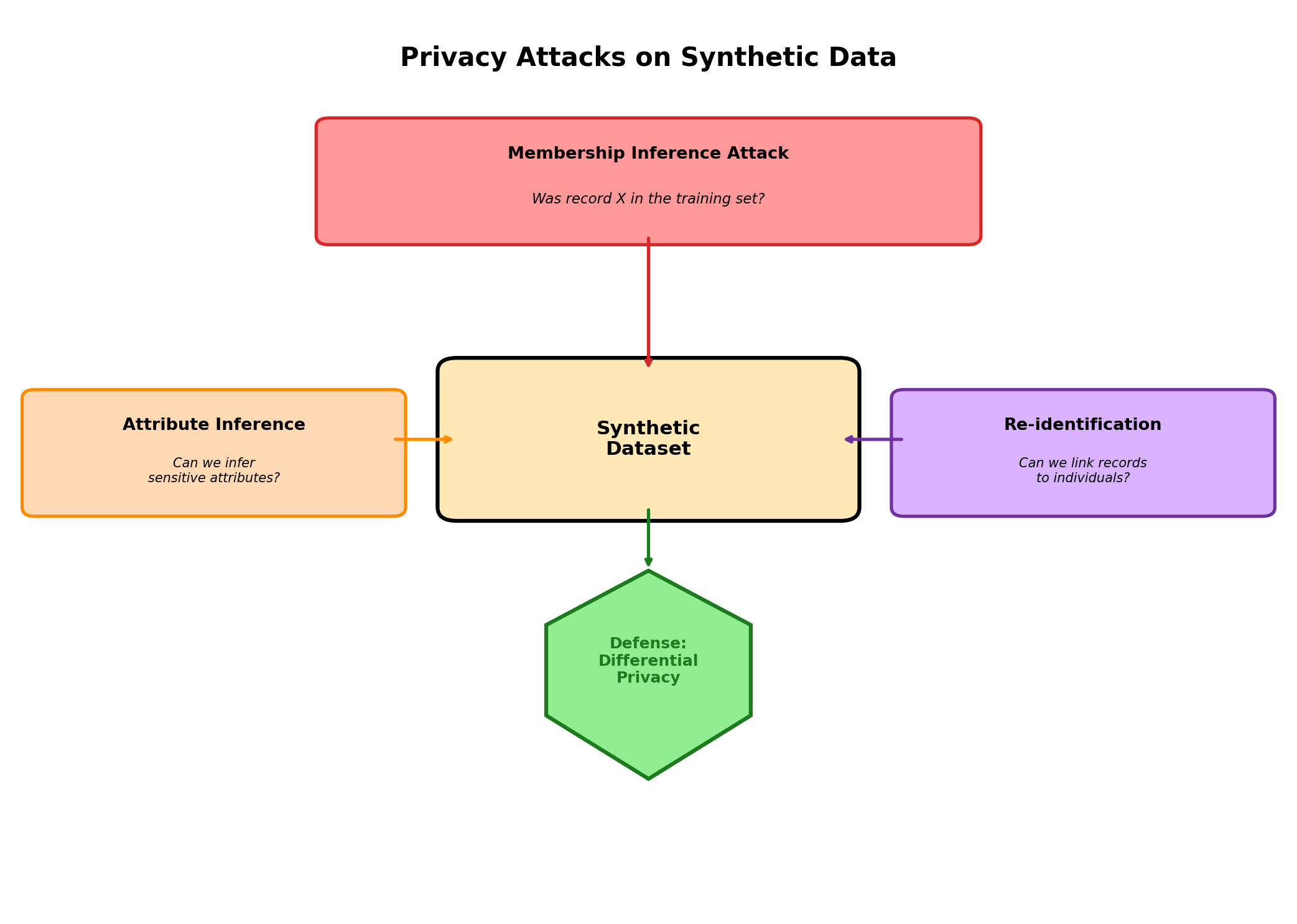
8.2 Privacy Attack Models

To evaluate privacy risks in synthetic data, we must first understand how attackers think. Privacy attacks are methods for extracting sensitive information from models or datasets. Several canonical attacks illuminate the landscape:

Membership Inference Attacks

A membership inference attack asks: was this specific record in the training dataset? An attacker who can access the generator or model may probe it with known individuals and measure how differently it behaves. If a GAN produces unusually high-confidence outputs for records matching real training samples, or if a model's loss is systematically lower for training data, membership can be inferred.

Example: An attacker knows Alice's medical profile and queries a synthetic patient generator with Alice's attributes. If the generator produces Alice-like patients with improbably high fidelity, the attacker may infer that Alice was in the training cohort. This is particularly dangerous in medical privacy contexts where membership in a specific study or disease cohort is itself sensitive.

Attribute Inference Attacks

Rather than determining membership, an attribute inference attack deduces a sensitive attribute (e.g., diagnosis, income) from observable attributes. An attacker might observe that a synthetic dataset shows an unusually strong correlation between demographic variables and a sensitive outcome, allowing them to infer unobserved attributes of individuals they know.

Example: A lender uses synthetic loan data to train a model. The synthetic data preserves a correlation between zip code and loan default that was present in the real training set. An attacker matches a real borrower's neighborhood to the synthetic cohort, infers their likely credit risk, and adjusts their business accordingly.

Reconstruction Attacks

A reconstruction attack aims to recover actual records from a synthetic dataset. This is most dangerous when synthetic data is generated via a disclosure-prone method such as data swapping or partial synthesis. If a dataset reveals that Alice's age is between 40–50, Alice's zip code is 10023, and Alice's income is between 100k–120k, an attacker might cross-reference this narrow profile with public records and pinpoint a real individual.

Example: A researcher releases partially synthetic data where only age and income are synthetic but zip code and job title are real. An attacker combines the synthetic age/income with the real zip code and title, then queries voter registration or LinkedIn to narrow down the individual.

Linkage Attacks

A linkage attack combines synthetic data with external datasets to re-identify individuals. Even if synthetic data is fully fake, rare combinations of attributes may correspond to unique real individuals in the population.

Example: A synthetic dataset includes a 65-year-old female neurologist in rural Montana who loves curling. This combination is so rare in the population that an attacker can cross-reference publicly available datasets (medical directories, hobbies, demographics) and uniquely identify the real individual, even though the synthetic record was generated and not copied from the training set.

8.3 Measuring Privacy: Classical Approaches

Before differential privacy formalized privacy into mathematics, researchers used heuristic measures. These are still widely applied and useful for quick assessment, though they have significant limitations.

k-Anonymity

A dataset achieves k-anonymity if every record is indistinguishable from at least k–1 others in the dataset based on quasi-identifiers (attributes that, in combination, might identify individuals). If a dataset of patients achieves 5-anonymity on attributes {age, zip code, gender}, then every combination of age/zip/gender corresponds to at least 5 individuals in the dataset.

Achieving k-anonymity: Generalization and suppression. Generalize 41 years old to "40–50 years old," or replace exact zip codes with broader regions. The result is a dataset where rare combinations are masked.

Limitation: k-anonymity does not protect against attribute inference. If all 5 individuals with age "40–50," zip "10023," gender "F" are diabetic, an attacker who learns these quasi-identifiers can infer diabetes membership with high confidence. The dataset is k-anonymous but not privacy-protecting against attribute attacks.

l-Diversity

l-diversity requires that for each combination of quasi-identifiers, there are at least l distinct values of the sensitive attribute. If a quasi-identifier group of 5 patients includes 3 diabetics and 2 non-diabetics, the attribute has diversity 2 (two distinct values), providing some protection against attribute inference.

Limitation: l-diversity can be superficial. If a group of 5 patients has diagnoses {diabetes, diabetes, diabetes, diabetes, rare_disease}, it achieves l-diversity = 2, but the rare disease is still highly identifiable. Frequency-based attacks remain possible.

t-Closeness

t-closeness requires that the distribution of a sensitive attribute within each quasi-identifier group is within distance t (typically measured via Earth Mover's Distance or similar metrics) from the global distribution. This prevents localized skew in attribute distributions.

Advantage: More robust than l-diversity. If the global population is 10% diabetic, each quasi-identifier group should have approximately 10% diabetic, not 80%.

Limitation: t-closeness requires choosing t, an arbitrary threshold. Small t leads to heavy information loss; large t provides weak guarantees. Moreover, these metrics assume quasi-identifier attributes are known in advance, which is unrealistic as attackers may have unanticipated side information.

Why Classical Metrics Fell Short

All three classical metrics (k-anonymity, l-diversity, t-closeness) share a fundamental weakness: they are heuristic and offer no formal guarantee against arbitrary attacks with unknown side information. Composition and reuse are not addressed—if an attacker observes multiple releases of anonymized data, their inferences compound. These metrics spawned decades of research showing attacks that circumvented them despite their apparent protections.

8.4 Differential Privacy: Formal Definitions and Intuition

Differential privacy sidesteps the limitations of classical metrics by formalizing privacy as indistinguishability. The central idea: if an observer cannot distinguish between a world where Alice's data is in a dataset and a world where it is not, then Alice's privacy is protected.

The Formal Definition

A mechanism M is ε-differentially private if for any two adjacent datasets D and D' (differing in one record), and for any subset S of possible outputs:

P(M(D) ∈ S) ≤ e^ε · P(M(D') ∈ S)

In words: the probability that the mechanism produces an output in set S is at most e^ε times higher when Alice's record is in the dataset than when it is not. The parameter ε (epsilon) quantifies privacy: smaller ε means tighter indistinguishability and stronger privacy. Typical ranges are ε ∈ {0.1, 1, 10}; ε < 1 is considered strong privacy.

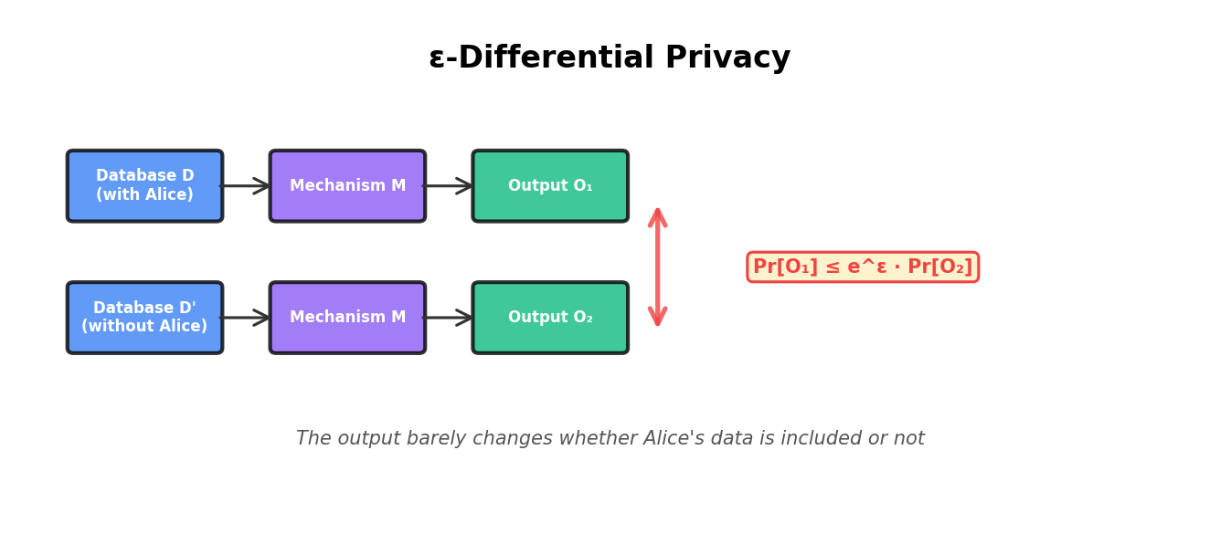
Intuition: Why This Works

The definition is clever because it makes no assumption about attacker knowledge or side information. An attacker observing any output cannot gain more than a factor of e^ε confidence about whether Alice's data was included. This holds even if the attacker has learned every other record in the dataset.

Example: Suppose a mechanism is 1-differentially private (ε = 1, so e^ε ≈ 2.7). An attacker observes an output and computes P(Alice ∈ dataset | output). Even in the worst case, this posterior probability is at most 2.7 times the prior P(Alice ∈ dataset). If the attacker started with a 1% prior, the posterior is at most 2.7%, a modest leak.

Composition: Privacy Under Reuse

A key advantage of differential privacy is principled composition. If you query a differentially private mechanism k times, the cumulative privacy cost is bounded. Sequential composition: If each of k queries is ε-DP, then the sequence is kε-DP. This means the dataset's total privacy budget is consumed by each use. You can make k queries before the privacy guarantee degrades.

8.5 Differential Privacy Mechanisms

How do we actually implement differential privacy? Several mechanisms add noise to data or queries, achieving indistinguishability.

Laplace Mechanism

The Laplace mechanism adds noise sampled from a Laplace distribution. For a query function f(D) that outputs a real number, the DP version returns f(D) + Lap(0, Δf/ε), where Δf is the sensitivity of f—the maximum change in output when a single record is added or removed.

Example: Query: "What is the average age in the dataset?" Over n records where ages are clipped to [a, b], the sensitivity is at most (b − a) / n (adding or removing a single record moves the mean by at most that amount). If ages are clipped to [0, 100], n = 10,000, and ε = 1, we add noise from Lap(0, 0.01) — negligible relative to the signal, but with a formal privacy guarantee. Whenever data is unbounded, you must pick a clipping range first; that choice — not the raw query — determines Δf.

Limitation: Laplace noise grows with sensitivity. For high-sensitivity queries (e.g., max value, which has sensitivity = max possible range), the noise overwhelms the signal, making the answer useless. Laplace is best for low-sensitivity queries like counts, sums, and averages.

Gaussian Mechanism

The Gaussian mechanism adds noise from a Gaussian distribution: f(D) + N(0, σ²) with σ = √(2 ln(1.25/δ)) · Δf / ε, so the variance scales as 2 ln(1.25/δ) · (Δf)² / ε². It achieves the relaxed guarantee known as (ε, δ)-differential privacy, which allows a failure probability δ (typically 10⁻⁵ to 10⁻⁷). In exchange for that small failure probability, the noise scale can be lower than Laplace for comparable ε and composition bounds are tighter.

Advantage: For repeated queries, Gaussian mechanism's composition is more favorable than Laplace. Many practical systems use Gaussian noise because the DP-SGD framework (discussed below) relies on it.

Exponential Mechanism

For queries with discrete outputs (e.g., "Which category is the mode?"), the exponential mechanism samples from a distribution proportional to exp(ε · f(candidate) / (2 · Δf)), where candidates are ranked by utility function f. High-utility options are sampled with higher probability, but the mechanism ensures indistinguishability across adjacent datasets.

Use case: Selecting the best machine learning model (from a finite set) in a privacy-respecting manner. The mechanism returns the best model but adds sufficient randomness to achieve DP.

Python Example: Laplace Mechanism

import numpy as np

def laplace_mechanism(query_result, sensitivity, epsilon):
    """
    Apply Laplace mechanism for DP.

    Args:
        query_result: The true result of the query (e.g., count, average).
        sensitivity: Maximum change in query result when one record added/removed.
        epsilon: Privacy parameter (smaller = stronger privacy).

    Returns:
        Noisy query result, differentially private.
    """
    scale = sensitivity / epsilon
    noise = np.random.laplace(loc=0, scale=scale)
    return query_result + noise

def gaussian_mechanism(query_result, sensitivity, epsilon, delta=1e-5):
    """
    Apply Gaussian mechanism for (epsilon, delta)-DP.
    """
    sigma = np.sqrt(2 * np.log(1.25 / delta)) * sensitivity / epsilon
    noise = np.random.normal(loc=0, scale=sigma)
    return query_result + noise

# Example: Count query on a dataset
# True count: 150 patients with diabetes
# Dataset size: 10,000 (so sensitivity of count = 1)
# Privacy: epsilon = 1

true_count = 150
sensitivity = 1
epsilon = 1

# Apply mechanisms
dp_count_laplace = laplace_mechanism(true_count, sensitivity, epsilon)
dp_count_gaussian = gaussian_mechanism(true_count, sensitivity, epsilon)

print(f"True count: {true_count}")
print(f"DP count (Laplace, ε=1): {dp_count_laplace:.1f}")
print(f"DP count (Gaussian, ε=1): {dp_count_gaussian:.1f}")

# Simulate multiple queries to show composition
budget = 1.0  # Total privacy budget
num_queries = 5
epsilon_per_query = budget / num_queries

print(f"\nWith budget ε={budget} over {num_queries} queries:")
for i in range(num_queries):
    dp_result = laplace_mechanism(true_count, sensitivity, epsilon_per_query)
    print(f"  Query {i+1}: {dp_result:.1f} (each query uses ε={epsilon_per_query:.2f})")

The example demonstrates composition: dividing a fixed budget across multiple queries shrinks the noise budget per query, increasing noise magnitude. This is the fundamental trade-off: more queries at lower privacy cost per query means noisier answers.

8.6 DP-SGD: Differentially Private Machine Learning

Synthetic data generation requires training models on potentially sensitive data. Differential Privacy Stochastic Gradient Descent (DP-SGD) enables training deep learning models while providing formal privacy guarantees.

Core Idea

Standard SGD updates model parameters by taking steps in the direction of gradients computed from training data. DP-SGD clips the gradient norm per sample, adds Gaussian noise, and uses carefully chosen batch sizes and learning rates to achieve differential privacy while preserving convergence.

The algorithm:

1. For each batch of B examples:
   1. Compute gradient for each example separately (not averaged).
   2. Clip each gradient to norm ≤ C (bounded sensitivity).
   3. Average clipped gradients.
   4. Add Gaussian noise with scale proportional to C / ε.
   5. Update parameters.
2. Track privacy budget: each pass through the data consumes ε from the total budget.

Why DP-SGD Works

By clipping gradients, we bound the sensitivity of the gradient update with respect to any single record. A record's presence or absence changes the average clipped gradient by at most C / B (in expectation). Adding Gaussian noise proportional to this sensitivity makes the update indistinguishable across adjacent datasets.

Practical Considerations

Hyperparameter tuning: Larger clip norm C preserves more gradient information but increases sensitivity. Smaller ε improves privacy but increases noise. Larger batch sizes B reduce per-sample gradient impact, improving privacy for the same ε. But larger batches may hurt generalization and increase training time.

Epochs and composition: DP-SGD's privacy cost depends on the number of epochs (passes through the data). If you train for 50 epochs with ε = 0.1 per epoch, the total privacy budget is 5. Many practitioners use advanced composition theorems (Rényi, concentrated DP) to improve this; the Opacus library (PyTorch) and TensorFlow Privacy implement optimized composition.

Python Example with Opacus

import torch
import torch.nn as nn
import torch.optim as optim
from torch.utils.data import DataLoader, TensorDataset
from opacus import PrivacyEngine

# Simple model for tabular data
class SimpleClassifier(nn.Module):
    def __init__(self, input_dim=10):
        super().__init__()
        self.net = nn.Sequential(
            nn.Linear(input_dim, 64),
            nn.ReLU(),
            nn.Linear(64, 32),
            nn.ReLU(),
            nn.Linear(32, 2)  # Binary classification
        )

    def forward(self, x):
        return self.net(x)

def train_with_dp(X_train, y_train, epsilon=1.0, delta=1e-5, epochs=10):
    """
    Train a model with differential privacy using DP-SGD.

    Args:
        X_train: Training features (n_samples, n_features)
        y_train: Training labels (n_samples,)
        epsilon: Privacy parameter
        delta: Failure probability
        epochs: Number of training epochs

    Returns:
        Trained model, privacy engine for tracking budget
    """
    # Prepare data
    dataset = TensorDataset(
        torch.FloatTensor(X_train),
        torch.LongTensor(y_train)
    )
    loader = DataLoader(dataset, batch_size=32, shuffle=True)

    # Initialize model and optimizer
    device = torch.device('cpu')
    model = SimpleClassifier(input_dim=X_train.shape[1]).to(device)
    optimizer = optim.Adam(model.parameters(), lr=0.001)

    # Attach DP engine
    privacy_engine = PrivacyEngine()
    model, optimizer, loader = privacy_engine.make_private(
        module=model,
        optimizer=optimizer,
        data_loader=loader,
        noise_multiplier=1.0,  # Controls noise scale
        max_grad_norm=1.0,     # Gradient clipping threshold
    )

    # Training loop
    criterion = nn.CrossEntropyLoss()

    for epoch in range(epochs):
        losses = []
        for X_batch, y_batch in loader:
            X_batch, y_batch = X_batch.to(device), y_batch.to(device)

            # Forward + backward
            logits = model(X_batch)
            loss = criterion(logits, y_batch)

            optimizer.zero_grad()
            loss.backward()
            optimizer.step()

            losses.append(loss.item())

        # Check privacy budget
        epsilon_used, best_alpha = privacy_engine.get_epsilon(delta)
        print(f"Epoch {epoch+1}/{epochs} | Loss: {np.mean(losses):.4f} | "
              f"ε used: {epsilon_used:.2f}")

        if epsilon_used > epsilon:
            print(f"Privacy budget exhausted (ε={epsilon}). Stopping training.")
            break

    return model, privacy_engine

# Example: Synthetic training data
np.random.seed(42)
X_train = np.random.randn(1000, 10)
y_train = (X_train[:, 0] + X_train[:, 1] > 0).astype(int)

# Train with DP
model, privacy_engine = train_with_dp(X_train, y_train, epsilon=1.0, epochs=10)

This example demonstrates DP-SGD training using Opacus, PyTorch's privacy library. The PrivacyEngine wraps the model and optimizer, implementing gradient clipping and noise addition automatically. The key function get_epsilon(delta) tracks cumulative privacy cost.

8.7 Generating Synthetic Data with Differential Privacy

Armed with DP fundamentals, we can now integrate privacy into synthetic data generation. There are several approaches, each with distinct trade-offs.

DP-CTGAN and DP-Generative Models

DP-CTGAN applies DP-SGD to training a CTGAN (Conditional Tabular GAN), a neural network designed for generating tabular data. The generator learns the distribution of real data while providing formal privacy guarantees. The privacy cost is the cumulative DP-SGD budget across all training epochs.

Trade-off: DP noise reduces generator training efficacy, leading to lower-fidelity synthetic data. Extensive empirical work shows that DP-CTGAN with strict privacy (ε < 1) often produces synthetic data with noticeably lower utility than non-private baselines. However, at looser privacy levels (ε ≈ 5–10), utility degradation is manageable.

DP-CTGAN Example

"""
DP-CTGAN (Differentially Private CTGAN)
Demonstrates training a privacy-preserving synthetic data generator.
"""
import pandas as pd
import numpy as np

# Simulate a small tabular dataset (real data)
np.random.seed(42)
n_samples = 500

real_data = pd.DataFrame({
    'age': np.random.normal(45, 15, n_samples),
    'income': np.random.normal(70000, 30000, n_samples),
    'purchased': np.random.binomial(1, 0.4, n_samples),
    'credit_score': np.random.normal(700, 100, n_samples)
})

# Ensure realistic ranges
real_data['age'] = real_data['age'].clip(18, 80)
real_data['income'] = real_data['income'].clip(20000, 200000)
real_data['credit_score'] = real_data['credit_score'].clip(300, 850)

print("Real Data Summary:")
print(real_data.describe())

# In a full implementation, we would use a library like ctgan or synthpop
# with DP-SGD modifications. For illustration, we show a simplified
# privacy-aware generation approach.

def generate_dp_synthetic_data(real_data, n_synthetic=500, epsilon=1.0,
                               clip_bounds=None):
    """
    Pedagogical privacy-aware synthetic data generator.

    IMPORTANT: this example is meant to *illustrate* the mechanics of clipping
    and Laplace noise. It is not a hardened DP system: it does not handle
    composition across columns rigorously, ignores correlations, and assumes
    the bounds in `clip_bounds` are public/non-data-dependent. Production
    systems use CTGAN with DP-SGD, PATE, or vetted libraries such as Tumult
    Analytics, OpenDP, or Google's diff-privacy.
    """
    if clip_bounds is None:
        raise ValueError(
            "clip_bounds must be a dict {col: (low, high)} with PUBLIC bounds. "
            "Reading the min/max from the data itself is not differentially private."
        )

    missing_bounds = set(real_data.columns) - set(clip_bounds)
    if missing_bounds:
        raise ValueError(
            f"Missing public bounds for columns: {sorted(missing_bounds)}"
        )

    synthetic = pd.DataFrame()
    # Each column consumes epsilon/(2*ncols) for the mean and the same for the
    # std, so the total budget across columns sums to `epsilon` (basic
    # composition). For tighter accounting, use RDP / zCDP instead.
    n_cols = len(real_data.columns)
    eps_per_stat = epsilon / (2 * n_cols)

    for col in real_data.columns:
        low, high = clip_bounds[col]
        clipped = real_data[col].clip(low, high)
        if high <= low:
            raise ValueError(f"Invalid bounds for {col}: {(low, high)}")

        # Sensitivities under add/remove neighboring datasets:
        #   mean over n records: (high - low) / n
        #   std below uses a loose pedagogical scale proxy. In a production
        #   DP release, use a vetted bounded-variance mechanism instead.
        n = len(clipped)
        sensitivity_mean = (high - low) / n
        sensitivity_std = (high - low) / 2

        noisy_mean = clipped.mean() + np.random.laplace(
            0, sensitivity_mean / eps_per_stat
        )

        # Binary columns should be sampled as Bernoulli, not as clipped
        # Gaussian values cast back to int.
        observed_values = set(clipped.dropna().unique())
        if observed_values.issubset({0, 1}) and low == 0 and high == 1:
            noisy_p = float(np.clip(noisy_mean, 0, 1))
            synthetic[col] = np.random.binomial(1, noisy_p, n_synthetic)
            continue

        noisy_std = clipped.std() + np.random.laplace(
            0, sensitivity_std / eps_per_stat
        )

        synthetic[col] = np.random.normal(noisy_mean, max(noisy_std, 1e-6), n_synthetic)
        synthetic[col] = synthetic[col].clip(low, high)

    return synthetic.astype(real_data.dtypes)

# Public, non-data-dependent clipping bounds. In practice these come from
# domain knowledge (e.g., "age in [0, 120]"), not from real_data.min()/max().
clip_bounds = {
    'age': (18, 100),
    'income': (0, 500_000),
    'purchased': (0, 1),
    'credit_score': (300, 850),
}

synthetic_data = generate_dp_synthetic_data(
    real_data, n_synthetic=500, epsilon=1.0, clip_bounds=clip_bounds,
)

print("\nDP Synthetic Data Summary (ε=1.0):")
print(synthetic_data.describe())

# Compare distributions (visually or with metrics)
print("\nMean Comparison:")
print(f"Real:      age={real_data['age'].mean():.1f}, "
      f"income={real_data['income'].mean():.0f}")
print(f"Synthetic: age={synthetic_data['age'].mean():.1f}, "
      f"income={synthetic_data['income'].mean():.0f}")

This example shows a simplified DP synthetic data generation: add noise to distributional statistics before sampling. Production systems (e.g., CTGAN with DP-SGD) are more sophisticated but follow the same principle: integrate privacy constraints into the generative model's training.

PATE Framework: Private Aggregation of Teacher Ensembles

An alternative to DP-SGD is the PATE framework. Train multiple "teacher" models on disjoint subsets of sensitive data (no privacy constraint). Each teacher learns its subset well. Then, train a "student" model on synthetic or public data by having each teacher vote on unlabeled examples. The student's labels come from aggregating teacher votes with added noise (Laplace or Gaussian). The noise ensures that the student cannot infer properties of any single teacher's training data.

Advantage: PATE separates privacy (the aggregation step) from model performance (each teacher is trained without DP constraints). Teachers can be arbitrarily complex; only the aggregation needs to be private. This often yields better utility than DP-SGD on complex models.

Disadvantage: Requires dividing sensitive data among teachers, reducing each teacher's training data. This can hurt utility for small datasets or rare subgroups. Also, generating synthetic labels via voting may be noisier than direct DP training.

8.8 Regulatory Landscape

Privacy is not only a technical concern but a regulatory one. Organizations must understand legal frameworks and how synthetic data fits (or fails to fit) within them.

GDPR (General Data Protection Regulation)

The EU's GDPR applies to processing of personal data of EU residents, regardless of where the organization is located. Key rights: individuals can request access to their data, have it erased, and opt out of processing. Key obligations: organizations must document consent, minimize data collection, and protect against unauthorized access.

Synthetic data and GDPR: If synthetic data is generated from real personal data, it may fall under GDPR (considered a "processing" of personal data). The GDPR article 32 mandates technical measures including anonymization. However, the legal status of synthetic data is contested: is fully synthetic data (no record corresponds to a real person) truly "personal data" under GDPR? Courts and regulators are still clarifying. Safe practice: treat synthetic data generated from personal data as quasi-personal until proven anonymized (via formal privacy analysis).

HIPAA (Health Insurance Portability and Accountability Act)

HIPAA regulates health data in the US. Its privacy rule requires de-identification of patient records before sharing. De-identification can be achieved through two methods: (1) "Safe Harbor," removing 18 specific identifiers (names, dates, addresses, etc.), or (2) "Expert Determination," where a statistician or security expert certifies that the risk of re-identification is minimal.

Synthetic data and HIPAA: Fully synthetic patient data (generated without copying real records) may sidestep HIPAA if it does not contain any of the 18 protected identifiers and passes expert determination. However, synthetic data is not explicitly mentioned in HIPAA, creating regulatory ambiguity. Many healthcare organizations use differential privacy certificates alongside synthetic data to establish compliance confidence.

CCPA (California Consumer Privacy Act)

CCPA grants California residents rights to know what personal information companies collect, delete it, and opt out of sale. Enforcement is by California Attorney General and private right of action.

Synthetic data and CCPA: Like GDPR, CCPA's treatment of synthetic data is evolving. If synthetic data is "derived from" personal data of CCPA-covered residents, it may be considered personal information. Safest practice: demonstrate non-linkability and non-attributability through privacy analysis.

Practical Compliance Strategy

Documentation: Maintain detailed records of how synthetic data was generated, privacy parameters (ε, δ for DP), and validation results. This supports claims of compliance.

Privacy by Design: Integrate privacy considerations from the start. Do not generate synthetic data naively and hope it is private; plan privacy controls.

Third-party Assessment: For high-stakes domains (healthcare, finance), engage external experts to audit privacy guarantees. This provides both technical rigor and regulatory credibility.

8.9 Fairness & Bias in Synthetic Data

Synthetic data can be a powerful tool for fairness—or a subtle mechanism for amplifying bias. Understanding both risks and opportunities is essential.

How Synthetic Data Can Perpetuate Bias

Memorization of real-world biases: If training data reflects historical discrimination (e.g., hiring data where certain demographics were systematically passed over), a generative model learns those patterns and reproduces them in synthetic samples. The synthetic data "hallucinate" discriminatory outcomes that were never explicitly in the training set but implicit in its statistical structure.

Amplification through resampling: A GAN trained on imbalanced data (e.g., 90% positive cases, 10% negative) may exaggerate the imbalance when generating synthetic data, pushing it closer to 95% or 99% positive. This amplification can worsen model bias.

Privacy-utility trade-off: Synthetic data generated with strict differential privacy (ε < 1) is necessarily noisy and may lose minority subgroup structure. A dataset with 5% disabled individuals might see that minority group "smoothed away" by DP noise, making the synthetic data even less representative.

How Synthetic Data Can Mitigate Bias

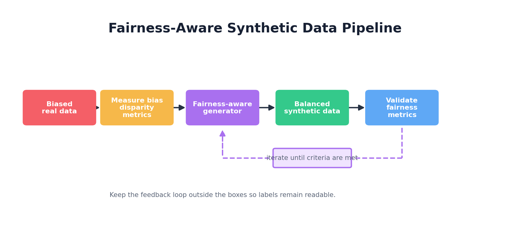
Controlled generation: Explicitly guide synthetic data generation to achieve target demographics. Instead of generating all 1 million records from a biased historical distribution, generate 500k records from the historical distribution and 500k with controlled demographics (e.g., 50% from each gender). This rebalanced synthetic data can help train fairer downstream models.

Counterfactual simulation: Use synthetic data to explore "what-if" scenarios. Generate a counterfactual dataset where a historically discriminatory policy is removed, or where protected attributes are randomized. Train models on this synthetic data to understand how they would behave under fairer conditions.

Bias detection: Generate synthetic data with known properties and audit generative models' fidelity across demographic groups. If a GAN produces high-fidelity synthetic data for majority groups but low-fidelity for minorities, this signals the generator's learned biases. Detecting bias in the generator allows you to refine it.

Fairness-Aware Synthetic Data Generation

Approach 1: Conditional generation by demographic. Train separate generators for each demographic group (e.g., gender), ensuring each learns its subgroup well. Then, sample synthetically from each generator in proportions that match your fairness goal (e.g., 50-50 gender, regardless of training data proportions).

Approach 2: Fairness constraints in the loss function. Add fairness terms to the generative model's loss. For example, penalize disparities in a sensitive attribute's distribution across demographic groups. The generator then balances fidelity against fairness.

Approach 3: Post-generation rebalancing. Generate synthetic data unconstrained, then resample or reweight records to achieve fairness targets. Keep records from underrepresented groups, downsample overrepresented groups. This is simple but loses some fidelity.

Python Example: Fairness-Aware Rebalancing

import pandas as pd
import numpy as np

# Synthetic dataset with gender imbalance
synthetic_data = pd.DataFrame({
    'age': np.random.normal(40, 15, 1000),
    'income': np.random.normal(70000, 25000, 1000),
    'gender': np.random.choice(['M', 'F'], 1000, p=[0.7, 0.3]),
    'hired': np.random.binomial(1, 0.5, 1000)
})

print("Original Synthetic Data Distribution:")
print(synthetic_data['gender'].value_counts(normalize=True))
print(f"Hired rate by gender:")
print(synthetic_data.groupby('gender')['hired'].mean())

# Fairness goal: balance gender 50-50
target_gender_dist = {'M': 0.5, 'F': 0.5}

# Rebalance via stratified resampling
rebalanced = []
for gender, target_proportion in target_gender_dist.items():
    subset = synthetic_data[synthetic_data['gender'] == gender]
    n_samples = int(len(synthetic_data) * target_proportion)
    sampled = subset.sample(n=n_samples, replace=True, random_state=42)
    rebalanced.append(sampled)

rebalanced_data = pd.concat(rebalanced, ignore_index=True)

print("\nRebalanced Synthetic Data Distribution:")
print(rebalanced_data['gender'].value_counts(normalize=True))
print(f"Hired rate by gender (post-rebalancing):")
print(rebalanced_data.groupby('gender')['hired'].mean())

# More sophisticated: check for hiring disparities and adjust
print("\nFairness Audit:")
m_hired_rate = synthetic_data[synthetic_data['gender'] == 'M']['hired'].mean()
f_hired_rate = synthetic_data[synthetic_data['gender'] == 'F']['hired'].mean()
disparity = abs(m_hired_rate - f_hired_rate)
print(f"Original hiring disparity: {disparity:.3f}")

m_hired_rate_rb = rebalanced_data[rebalanced_data['gender'] == 'M']['hired'].mean()
f_hired_rate_rb = rebalanced_data[rebalanced_data['gender'] == 'F']['hired'].mean()
disparity_rb = abs(m_hired_rate_rb - f_hired_rate_rb)
print(f"Rebalanced hiring disparity: {disparity_rb:.3f}")

if disparity_rb < disparity:
    print("Rebalancing reduced hiring disparity.")

This example shows how rebalancing synthetic data by demographic can reduce disparities. In practice, fairness may conflict with utility (perfectly balanced data may not match real-world distributions), requiring domain judgment to navigate trade-offs.

8.10 Hands-On: Adding Differential Privacy to a Generator

Let's build a complete example: take a simple synthetic data generator and wrap it with differential privacy using the diffprivlib library.

Setup and Basic Generator

"""
Hands-On: Differentially Private Synthetic Data Generation
Using diffprivlib (https://diffprivlib.readthedocs.io/)
"""

import numpy as np
import pandas as pd
from sklearn.datasets import make_classification
from sklearn.ensemble import RandomForestClassifier
from diffprivlib.models import LogisticRegression as DPLogisticRegression
# diffprivlib emits a `PrivacyLeakWarning` whenever a fit() call uses
# data-dependent bounds (which would silently break the DP guarantee).
# Promote those warnings to errors so they can never be ignored.
import warnings
from diffprivlib.utils import PrivacyLeakWarning
warnings.simplefilter("error", PrivacyLeakWarning)

# Step 1: Create a simple synthetic dataset (non-private baseline)
print("=== Non-Private Baseline ===")
X_train, y_train = make_classification(
    n_samples=1000,
    n_features=5,
    n_informative=3,
    n_redundant=2,
    random_state=42
)

# Train a simple classifier
clf_baseline = RandomForestClassifier(n_estimators=10, random_state=42)
clf_baseline.fit(X_train, y_train)
baseline_accuracy = clf_baseline.score(X_train, y_train)
print(f"Non-private model accuracy: {baseline_accuracy:.3f}")

# Step 2: Train a DP classifier
print("\n=== Differentially Private Model ===")
X_train_df = pd.DataFrame(X_train, columns=[f'feature_{i}' for i in range(5)])

dp_clf = DPLogisticRegression(
    epsilon=1.0,      # Privacy budget
    data_norm=2.0,    # Bounds on data
    random_state=42
)

try:
    dp_clf.fit(X_train, y_train)
    dp_accuracy = dp_clf.score(X_train, y_train)
    print(f"DP model accuracy (ε=1.0): {dp_accuracy:.3f}")
    print(f"Utility loss: {baseline_accuracy - dp_accuracy:.3f}")
except Exception as e:
    print(f"Note: {e}")
    # If exact fitting fails, we can still demonstrate the concept
    print("(In practice, DP model training requires careful tuning of parameters)")

# Step 3: Tighter privacy
print("\n=== Tighter Privacy (ε=0.5) ===")
dp_clf_tight = DPLogisticRegression(
    epsilon=0.5,
    data_norm=2.0,
    random_state=42
)

try:
    dp_clf_tight.fit(X_train, y_train)
    dp_accuracy_tight = dp_clf_tight.score(X_train, y_train)
    print(f"DP model accuracy (ε=0.5): {dp_accuracy_tight:.3f}")
    print(f"Utility loss: {baseline_accuracy - dp_accuracy_tight:.3f}")
    print("(Tighter privacy yields lower utility, as expected)")
except Exception as e:
    print(f"Note: {e}")

print("\n=== Privacy Budget Interpretation ===")
print("ε = 1.0 allows ~2.7x confidence gain per query")
print("ε = 0.5 allows ~1.6x confidence gain per query")
print("Lower ε = stronger privacy (but lower utility)")

Advanced Example: DP-Aware Synthetic Data Pipeline

"""
Complete pipeline: Generate DP synthetic data, validate privacy, audit fairness.
"""

def generate_dp_synthetic_population(real_data, bounds, epsilon=1.0, n_synthetic=500):
    """
    Generate synthetic data with (a pedagogical version of) differential privacy.

    `bounds` must be a dict {col: (low, high)} derived from PUBLIC knowledge,
    not from real_data itself. Deriving bounds from the data would leak
    information about the extremes.

    Simple approach: estimate per-column mean and std with Laplace noise,
    then sample from a Gaussian with those parameters. Marginals only — this
    generator does NOT preserve correlations. For production use, prefer
    CTGAN+DP-SGD, PATE, or OpenDP/Tumult Analytics.
    """
    synthetic_records = []
    eps_per_feature = epsilon / (2 * len(real_data.columns))  # mean + std per col

    for feature_col in real_data.columns:
        low, high = bounds[feature_col]
        # Clip to the public bounds before computing any statistic so
        # sensitivity is controlled.
        clipped = np.clip(real_data[feature_col].values, low, high)
        n = len(clipped)

        # Sensitivities under add/remove neighboring datasets:
        sens_mean = (high - low) / n
        sens_std = (high - low) / 2

        mean_noisy = np.mean(clipped) + np.random.laplace(
            0, sens_mean / eps_per_feature
        )
        std_noisy = np.std(clipped) + np.random.laplace(
            0, sens_std / eps_per_feature
        )

        synthetic_col = np.random.normal(mean_noisy, max(std_noisy, 1e-6), n_synthetic)
        synthetic_col = np.clip(synthetic_col, low, high)  # clip to PUBLIC bounds
        synthetic_records.append(synthetic_col)

    return pd.DataFrame(
        np.column_stack(synthetic_records), columns=real_data.columns
    )

# Create synthetic real data (simulating a sensitive dataset)
np.random.seed(42)
real_df = pd.DataFrame({
    'age': np.random.normal(40, 12, 200),
    'income': np.random.normal(60000, 25000, 200),
    'score': np.random.normal(700, 50, 200),
})
real_df['age'] = real_df['age'].clip(18, 80)
real_df['income'] = real_df['income'].clip(20000, 150000)
real_df['score'] = real_df['score'].clip(300, 850)

# PUBLIC bounds (domain-derived — NOT computed from real_df itself).
public_bounds = {
    'age': (18, 80),
    'income': (20_000, 150_000),
    'score': (300, 850),
}

print("Real Data Statistics:")
print(real_df.describe())

# Generate DP synthetic data at two epsilon levels
synthetic_loose = generate_dp_synthetic_population(
    real_df, public_bounds, epsilon=10.0, n_synthetic=200,
)
synthetic_tight = generate_dp_synthetic_population(
    real_df, public_bounds, epsilon=1.0, n_synthetic=200,
)

print("\nDP Synthetic Data (ε=10.0, loose privacy):")
print(synthetic_loose.describe())

print("\nDP Synthetic Data (ε=1.0, tight privacy):")
print(synthetic_tight.describe())

# Measure utility degradation
from scipy.stats import ks_2samp

print("\n=== Privacy-Utility Trade-off ===")
for col in real_df.columns:
    stat_loose, p_loose = ks_2samp(real_df[col], synthetic_loose[col])
    stat_tight, p_tight = ks_2samp(real_df[col], synthetic_tight[col])
    print(f"{col}:")
    print(f"  ε=10.0: KS distance={stat_loose:.3f}")
    print(f"  ε=1.0:  KS distance={stat_tight:.3f}")

print("\nObservation: Tighter privacy (lower ε) leads to greater distribution shift.")

This hands-on example demonstrates the privacy-utility frontier: as ε decreases (stronger privacy), the synthetic data diverges more from the real distribution (lower utility). Practitioners must navigate this trade-off based on their specific needs and constraints.

Conclusion

Privacy and fairness in synthetic data generation are non-negotiable concerns. Synthetic data is a powerful tool for unlocking data utility while respecting individual privacy—but only if built with rigor.

The journey from classical privacy metrics (k-anonymity, l-diversity) to differential privacy represents a fundamental shift: from heuristics to mathematics. Differential privacy formalizes privacy as indistinguishability, providing formal guarantees that hold against arbitrary attacks with unknown side information. Mechanisms like Laplace noise, Gaussian noise, and the exponential mechanism are the technical workhorses. DP-SGD and PATE enable training deep learning models (including generative models) while maintaining privacy.

Integrating differential privacy into synthetic data generation—via DP-CTGAN, DP-VAE, or custom pipelines—is now mainstream. The challenge is navigating the privacy-utility-fairness triangle: as privacy tightens, utility often degrades. As we enforce fairness (rebalancing demographics), we may introduce bias or reduce fidelity. There are no one-size-fits-all solutions; each application requires domain judgment, stakeholder input, and rigorous validation.

Regulators (GDPR, HIPAA, CCPA) are gradually clarifying synthetic data's legal status, but ambiguity persists. Best practice is to treat synthetic data generated from personal data as quasi-personal until proven private, and to engage legal counsel early.

With careful design, audit, and transparency, synthetic data can become a trusted tool for democratizing data access without sacrificing individual privacy or collective fairness.