1. Why Tabular Data Is Special
Tabular data—the rows and columns of spreadsheets, databases, and data warehouses—is arguably the most important data type for enterprise and research. Unlike images or text, tabular data embodies structured business logic: customer records with demographics, transaction histories, medical histories with diagnoses and treatments, financial portfolios, sensor measurements with timestamps. It's also the hardest to synthesize well.
Why? Three reasons. First, tabular data mixes fundamentally different data types in a single table: continuous variables (income, age, temperature), categorical variables (gender, country, product type), ordinal variables (education level, star ratings), and increasingly, temporal features and structured embeddings. A single method cannot handle all four.
Second, columns are bound by complex correlations and business constraints. Age and retirement income are correlated; a customer's ZIP code constrains their state; purchase amount scales with customer tenure; a diagnosis constrains which treatments are valid. Real-world tables encode decades of business rules and statistical patterns. Naive synthetic data violates these constraints, making it useless downstream.
Third, tabular data often exists in hierarchical, multi-table structures with foreign keys. A customer table links to orders, which link to line items; a hospital database has patients, admissions, diagnoses, and medications with intricate referential integrity rules. Synthesizing one table in isolation breaks these relationships, destroying the utility of the entire dataset.
This chapter covers the full spectrum of approaches—from classical copulas to hybrid methods combining copula theory with deep learning—and practical techniques for handling the messy realities of enterprise data.
2. Classical Approaches Revisited
Gaussian Copula
The Gaussian copula is the workhorse of classical tabular synthesis. Recall from Chapter 2: a copula is a function that couples marginal distributions into a joint distribution. The Gaussian copula uses a multivariate normal distribution to model correlations, then applies the inverse CDF of each column's empirical or parametric distribution.
The algorithm:
- Estimate the marginal distribution of each column (histogram for categorical, Gaussian or KDE for continuous).
- Transform each column to uniform [0, 1] using its empirical CDF: u_i = F_i(x_i).
- Transform uniform samples to Gaussian: z_i = Φ^{-1}(u_i).
- Estimate the correlation matrix Σ of the Gaussian-transformed data.
- To generate: sample from N(0, Σ), apply Φ to get uniforms, apply inverse CDFs to recover original scales.
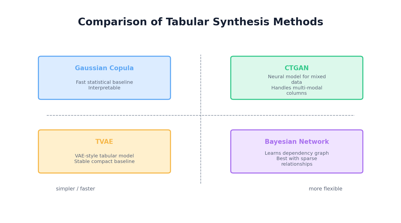
Strengths: Fast, interpretable, preserves marginals by construction, no hyperparameters. Weaknesses: assumes the Gaussian copula is adequate (it's not for highly non-linear relationships), categorical variables are treated as continuous (problematic for high-cardinality columns), and it cannot model complex multimodal or skewed distributions without augmentation.
Bayesian Networks for Tabular Data
Bayesian networks model dependencies as a directed acyclic graph (DAG): nodes are variables, edges represent conditional dependencies. To generate: sample parents first, then condition children on parent values. This respects causal structure and handles mixed data types naturally.
Example: a simple BN might have age → income (age influences income), education → income, and income → debt. To sample, draw age, education, then income conditioned on both, then debt conditioned on income.
Learning a BN from data involves: (1) structure learning—discovering the DAG, (2) parameter learning—estimating conditional probability tables (CPTs) or continuous conditional distributions. For tabular data, algorithms like constraint-based (PC algorithm) or score-based (hill-climbing) structure learning work well.
Both classical approaches scale to dozens of columns but struggle with high-cardinality variables, complex multimodal distributions, and subtle non-linear correlations. For larger, messier datasets, deep learning methods take over.
3. CTGAN — Conditional GAN for Tabular Data
The Architecture
CTGAN (Conditional Generative Adversarial Network for Tabular data), introduced by Xu et al. at NeurIPS 2019, is a GAN specifically engineered for mixed-type tabular synthesis. It is bundled in the open-source Synthetic Data Vault (SDV) library and has become one of the most widely used baselines for tabular synthesis in industry practice.
The key innovation: mode-specific normalization. Categorical columns are one-hot encoded and fed to a discriminator that sees sparse, discrete signals. Continuous columns are normalized, but different columns may have vastly different scales and distributions. Naive approaches feed these directly to a discriminator, which struggles because early discriminators easily classify samples as fake based on scale alone.
CTGAN's solution: for each continuous column, apply a VGM (Variational Gaussian Mixture) transform. Fit a Gaussian mixture to the column, then normalize by whichever mode is most likely given the sample's value. This "de-scales" the data so that a discriminator focuses on realistic joint patterns, not individual column ranges.
Mathematically, for a sample x from a column with m modes:
# Fit GMM offline: p(x) = Σ_k w_k * N(μ_k, σ_k)
# For new sample x, compute responsibility: r_k = w_k * N(x | μ_k, σ_k) / p(x)
# Normalize: x_norm = (x - μ_argmax_k(r_k)) / σ_argmax_k(r_k)
# Now x_norm is approximately N(0, 1) regardless of original scale
The generator and discriminator are standard MLPs. The generator takes latent noise and samples from a categorical embedding table for categorical columns. The discriminator is a standard classifier. Both are trained adversarially.

Training-by-Sampling
Another innovation: training-by-sampling. CTGAN selects a discrete column and category as a condition, then trains the generator to produce rows matching that condition. Categories are sampled with a log-frequency weighting, so rare categories appear often enough during training without making every class artificially uniform. This gives the discriminator and generator repeated exposure to minority categories while still preserving information about their real frequencies.
SDV Implementation
The Synthetic Data Vault (SDV) library makes CTGAN accessible. Here's a complete example:
from sdv.single_table import CTGANSynthesizer
from sdv.metadata import Metadata
import pandas as pd

# Load data
df = pd.read_csv('customer_data.csv')
# Columns: age (int), income (float), country (str), purchased (bool)

# Detect metadata and train
metadata = Metadata.detect_from_dataframe(data=df)
synthesizer = CTGANSynthesizer(metadata, epochs=300, batch_size=32)
synthesizer.fit(df)

# Generate synthetic data
synthetic_df = synthesizer.sample(num_rows=5000)

# Evaluate: compare distributions. Current SDV releases ship evaluation via
# the standalone `sdmetrics` package, not `sdv.metrics.tabular`.
from sdmetrics.single_table import CSTest, KSComplement
cs_score = CSTest.compute(real_data=df, synthetic_data=synthetic_df, metadata=metadata)
ks_score = KSComplement.compute(real_data=df, synthetic_data=synthetic_df, metadata=metadata)
print(f"CSTest (categorical similarity): {cs_score:.3f}")
print(f"KSComplement (continuous similarity): {ks_score:.3f}")
Under the hood, SDV:
- Detects column types (categorical, numeric, datetime).
- Fits a Bayesian metadata table describing each column (unique values, distribution type, missing value percentage).
- Normalizes continuous columns using mode-specific scaling.
- One-hot encodes categorical columns.
- Trains CTGAN generator and discriminator on the preprocessed data.
- When sampling, generates fake data, applies inverse transformations, and returns a DataFrame.
CTGAN excels at capturing complex dependencies and handling mixed types. However, training is slower than classical methods (hours for large datasets), and hyperparameter tuning (learning rate, batch size, epochs) is often needed for optimal results.
4. TVAE — Tabular Variational Autoencoder
TVAE is an alternative to CTGAN using a VAE architecture instead of adversarial training. It often trains faster and more stably, though sample quality can be slightly lower.
The TVAE encoder compresses tabular data to a latent vector, then the decoder reconstructs. Categorical columns are one-hot encoded and reconstructed with a softmax head trained under cross-entropy; continuous columns are mode-specifically normalized (the same VGM transform used by CTGAN) and reconstructed under a Gaussian likelihood. The loss combines reconstruction (Gaussian log-likelihood for continuous modes, cross-entropy for categoricals) with the usual KL term to a standard-normal prior.
A key architectural contrast: it is CTGAN, not TVAE, that uses the Gumbel-Softmax trick — specifically in its generator head, where a soft, differentiable relaxation of the categorical argmax is needed so adversarial gradients can flow through discrete outputs. TVAE sidesteps the issue because its reconstruction loss operates directly on the softmax probabilities, so standard backprop suffices.
SDV usage is nearly identical:
from sdv.single_table import TVAESynthesizer
from sdv.metadata import Metadata

metadata = Metadata.detect_from_dataframe(data=df)
synthesizer = TVAESynthesizer(metadata, epochs=300, batch_size=32)
synthesizer.fit(df)
synthetic_df = synthesizer.sample(num_rows=5000)
CTGAN vs. TVAE: When to Use Which?
| Criterion | CTGAN | TVAE |
|---|---|---|
| Sample Quality | Typically excellent | Good; can be blurry for rare classes |
| Training Stability | Can be unstable (adversarial training) | More stable |
| Training Speed | Slower (two networks) | Faster |
| Handling Imbalance | Better (training-by-sampling) | Weaker; requires post-processing |
| Rare Categories | Learns better with oversampling | Tends to miss rare classes |
| Hyperparameter Tuning | Requires careful tuning | Less tuning needed |
In practice, start with TVAE for speed; switch to CTGAN if you need higher quality or better rare-class coverage.
5. CopulaGAN — Marrying Copulas and Deep Learning
CopulaGAN, a variant shipped with SDV, combines the ideas of Gaussian copulas and CTGAN. Rather than running two independent models, it inserts a copula-style pre-processing step in front of an otherwise standard CTGAN.
The Algorithm
- Marginal CDFs: For each continuous column, fit its empirical (or parametric) marginal CDF Fi.
- Copula transform: Map every continuous column through Φ-1(Fi(xi)), producing a table whose continuous marginals are (approximately) standard normal. Categorical columns are left to CTGAN's usual one-hot handling.
- CTGAN on the transformed table: Train a CTGAN on the copula-transformed data. Because the continuous columns are now well-behaved, the adversarial game is stabilised.
- Sampling: Draw synthetic rows from the CTGAN and invert the copula transform (xi = Fi-1(Φ(zi))) so each column recovers its original marginal distribution.
Strengths: the pre-transform fixes the marginal distributions exactly while CTGAN learns the joint dependence structure on the transformed scale. Weaknesses: a second set of hyperparameters (distribution families for each marginal) must be chosen, and on real datasets the quality gain over plain CTGAN is often modest.
SDV includes CopulaGAN:
from sdv.single_table import CopulaGANSynthesizer
from sdv.metadata import Metadata

metadata = Metadata.detect_from_dataframe(data=df)
synthesizer = CopulaGANSynthesizer(metadata, epochs=100)
synthesizer.fit(df)
synthetic_df = synthesizer.sample(num_rows=5000)
CopulaGAN is best when you want stronger control over marginal modeling and have time for two-stage training. For most practitioners, CTGAN or TVAE suffice.
6. Bayesian Networks — Structure and Sampling
Bayesian networks offer a different philosophy: explicit conditional independence structure. This is valuable when you understand your data's causal or logical structure.
Structure Learning and Parameter Learning
A BN is a DAG where nodes are variables and edges represent "X influences Y." To sample: topologically sort, then sample each node conditioned on its parents.
Structure learning can be done via:
- Constraint-based (PC algorithm): Uses conditional independence tests (e.g., chi-squared for categorical data) to infer which edges are absent.
- Score-based (hill-climbing): Searches over DAGs, scoring each by BIC or likelihood. Greedy but practical.
- Expert knowledge: Often the best: domain experts know the structure. Encode it directly.
For parameter learning, estimate each node's CPT (conditional probability table) from data, or fit a continuous conditional distribution (e.g., linear regression for continuous children).
pgmpy Example
The pgmpy library (Probabilistic Graphical Models in Python) implements BN structure and parameter learning:
from pgmpy.models import BayesianNetwork
from pgmpy.estimators import MaximumLikelihoodEstimator, BayesianEstimator
from pgmpy.factors.discrete import TabularCPD
import pandas as pd

# Load data
df = pd.read_csv('customer_data.csv')

# Define structure (DAG): age -> income, education -> income
model = BayesianNetwork([
    ('age', 'income'),
    ('education', 'income'),
    ('income', 'debt')
])

# Learn parameters from data
model.fit(df, estimator=MaximumLikelihoodEstimator)

# Check learned CPD for income
print(model.get_cpds('income'))

# Sample
samples = model.sample(size=5000)
The downside: if your data has 50 columns, structure learning becomes intractable. BNs scale well for 10-20 variables with domain expertise; beyond that, deep learning approaches are more practical.
7. Handling Challenges in Real-World Tabular Data
Missing Values
Real datasets have missing data (NaNs, NULLs). SDV handles this by encoding missingness as a separate column during training. For example, if column income has 15% missing, SDV creates an auxiliary binary column income__is_missing with 85% zeros and 15% ones. The model learns to correlate this missingness pattern with other variables (e.g., income is missing for non-US customers).
When sampling, if a synthetic row has income__is_missing = 1, the income value is set to NaN in the output DataFrame.
from sdv.single_table import CTGANSynthesizer
from sdv.metadata import Metadata

# SDV automatically detects and handles NaNs
metadata = Metadata.detect_from_dataframe(data=df)
synthesizer = CTGANSynthesizer(metadata)
synthesizer.fit(df)  # df contains NaN values
synthetic_df = synthesizer.sample(num_rows=5000)
# synthetic_df preserves NaN patterns from original data
Imbalanced Categories
If a categorical column has one dominant class (e.g., 98% "no" and 2% "yes"), the generator may almost always produce the dominant class. Solutions:
- Conditional sampling: Generate data conditioned on the rare class. See Section 9.
- Post-processing: Resample the synthetic data to match target class distributions.
- CTGAN training-by-sampling: Already helps by oversampling rare classes during training. Increase the oversampling ratio.
High-Cardinality Columns
A column like customer_id or product_sku with thousands of unique values poses challenges: the model must learn a categorical distribution over 10,000+ classes. One-hot encoding becomes infeasible.
Solutions:
- Drop or anonymize: Exclude IDs from synthesis, generate new random IDs post-hoc.
- Embeddings: Learn low-dimensional embeddings for each category (like word embeddings in NLP), then embed/de-embed during generation.
- Coarsen: Group rare categories into "other" or aggregate to parent level (e.g., product family instead of product SKU).
Temporal Ordering and Sequences
Some tables are naturally ordered (e.g., bank transactions sorted by timestamp, or a time series table with one row per day). Standard tabular methods treat rows as i.i.d., losing temporal structure.
For sequences, use methods designed for temporal data: RNNs, Transformers, or dedicated synthetic sequence libraries. For table rows that happen to have a timestamp, include the timestamp as a column; SDV will learn temporal correlations if they exist in the data.
Referential Integrity in Multi-Table Datasets
Enterprise databases have multiple tables with foreign keys. A customer table has customer_id; an orders table has customer_id and order_id; a line_items table has order_id. To synthesize, you must preserve these keys: every order's customer_id must exist in the synthetic customers table.
Naive approaches synthesize each table independently, breaking referential integrity. SDV solves this via HMA (Hierarchical Modeling Approach), covered in Section 8.
8. Multi-Table Synthesis — HMA and Foreign Key Preservation
Many real-world datasets are relational: orders belong to customers, line items belong to orders. Synthesizing one table breaks relationships with others. SDV's HMA approach synthesizes the entire relational structure coherently.
Hierarchical Modeling Approach (HMA)
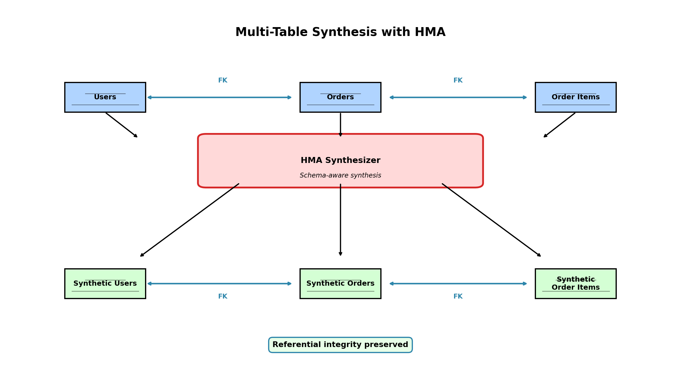
HMA treats a multi-table dataset as a hierarchy. Tables are ordered by dependency: synthesize the "root" table (e.g., customers) first, then synthesize child tables while preserving foreign-key relationships and learned parent-child patterns.
- Metadata specification: Define relationships (foreign keys) between tables.
- Root table synthesis: Model the root table with HMA's table-level statistical model and generate synthetic parent rows.
- Child table synthesis: Model child rows together with relationship and cardinality information, then sample child rows connected to synthetic parents.
- Repeat recursively: Continue through supported hierarchy levels, keeping primary and foreign keys coherent.
HMA with SDV
from sdv.multi_table import HMASynthesizer
from sdv.metadata import Metadata
import pandas as pd

# Load multiple tables
customers_df = pd.read_csv('customers.csv')  # Columns: customer_id, age, country
orders_df = pd.read_csv('orders.csv')  # Columns: order_id, customer_id, amount, date

# Create metadata from the table dictionary
metadata = Metadata.detect_from_dataframes(data={
    'customers': customers_df,
    'orders': orders_df
})

# Train HMA
synthesizer = HMASynthesizer(metadata)
synthesizer.fit(data={
    'customers': customers_df,
    'orders': orders_df
})

# Sample
synthetic_data = synthesizer.sample()
# Result: Dict with 'customers' and 'orders' DataFrames
# Referential integrity is preserved: every order's customer_id exists in synthetic customers
synthetic_customers = synthetic_data['customers']
synthetic_orders = synthetic_data['orders']

# Verify integrity
customer_ids_present = set(synthetic_customers['customer_id'])
order_customer_ids = set(synthetic_orders['customer_id'])
assert order_customer_ids.issubset(customer_ids_present), "Foreign key violated!"
HMA is useful for enterprise applications because it preserves declared relationships and referential integrity, making synthetic data easier to use in downstream systems that expect connected tables.
9. Conditional Generation — Constraints and Targeted Synthesis
Sometimes you want synthetic data that satisfies specific conditions: generate premium customers from a given region, or oversample rare fraud labels while preserving the rest of the joint distribution. Conditional generation is key to balancing imbalanced classes and testing edge cases.
Conditional Sampling with SDV
from sdv.single_table import CTGANSynthesizer
from sdv.metadata import Metadata
from sdv.sampling import Condition

# Train on full data
metadata = Metadata.detect_from_dataframe(data=df)
synthesizer = CTGANSynthesizer(metadata)
synthesizer.fit(df)

# Generate rows with fixed attribute values
us_premium = Condition(
    num_rows=1000,
    column_values={
        'country': 'US',
        'is_premium': True
    }
)

samples = synthesizer.sample_from_conditions([us_premium])
Under the hood, SDV still has to honor feasibility. If the requested combination is extremely rare or impossible in the training data, sampling slows down or fails. That is a useful signal: the synthetic generator is telling you your requested slice may not exist in the source distribution.
Handling Imbalanced Classes
For a highly imbalanced binary outcome (fraud: 0.5%), generate synthetic fraud cases via conditional sampling:
normal_transactions = synthesizer.sample(num_rows=5000)  # Default, mostly non-fraud
fraud_condition = Condition(num_rows=50, column_values={'is_fraud': 1})
fraud_transactions = synthesizer.sample_from_conditions([fraud_condition])

# Combine
balanced_synthetic = pd.concat([normal_transactions, fraud_transactions], ignore_index=True)
This generates a dataset with a better fraud rate, useful for testing fraud detection models.
10. Hands-On: End-to-End Tabular Synthesis Pipeline
Here's a complete walkthrough: load a real dataset, fit multiple models (Copula, CTGAN, TVAE), generate synthetic data, and compare quality.
Complete Example: Iris Dataset
import pandas as pd
import numpy as np
from sdv.single_table import (
    GaussianCopulaSynthesizer,
    CTGANSynthesizer,
    TVAESynthesizer,
)
from sdv.metadata import Metadata
from sdmetrics.single_table import CSTest, KSComplement, TVComplement
from sklearn.datasets import load_iris
from sklearn.preprocessing import LabelEncoder
import warnings
warnings.filterwarnings('ignore')

# Step 1: Load and prepare data
# Using Iris for simplicity (in practice, use real enterprise data)
iris = load_iris()
df = pd.DataFrame(iris.data, columns=iris.feature_names)
df['species'] = iris.target_names[iris.target]

print("Original data shape:", df.shape)
print(df.head())

# Step 2: Split into train/test for fair evaluation
from sklearn.model_selection import train_test_split
train_df, test_df = train_test_split(df, test_size=0.2, random_state=42)
metadata = Metadata.detect_from_dataframe(data=train_df)

# Step 3: Train multiple models
print("\n--- Training models ---")

# Model 1: Gaussian Copula (classical baseline)
print("Training Gaussian Copula...")
copula_model = GaussianCopulaSynthesizer(metadata)
copula_model.fit(train_df)
copula_synthetic = copula_model.sample(num_rows=len(test_df))

# Model 2: CTGAN (modern GAN-based)
print("Training CTGAN...")
ctgan_model = CTGANSynthesizer(metadata, epochs=100, batch_size=32)
ctgan_model.fit(train_df)
ctgan_synthetic = ctgan_model.sample(num_rows=len(test_df))

# Model 3: TVAE (VAE-based)
print("Training TVAE...")
tvae_model = TVAESynthesizer(metadata, epochs=100, batch_size=32)
tvae_model.fit(train_df)
tvae_synthetic = tvae_model.sample(num_rows=len(test_df))

# Step 4: Evaluate using multiple metrics
print("\n--- Evaluation Results ---")

# sdmetrics single-table metrics are called as classmethods: Metric.compute(...)
metrics = {
    'CSTest': CSTest,
    'KSComplement': KSComplement,
    'TVComplement': TVComplement,
}

results = {}
for model_name, synthetic_df in [
    ('Gaussian Copula', copula_synthetic),
    ('CTGAN', ctgan_synthetic),
    ('TVAE', tvae_synthetic),
]:
    print(f"\n{model_name}:")
    results[model_name] = {}
    for metric_name, metric in metrics.items():
        try:
            score = metric.compute(
                real_data=test_df,
                synthetic_data=synthetic_df,
                metadata=metadata,
            )
            results[model_name][metric_name] = score
            print(f"  {metric_name}: {score:.4f}")
        except Exception as e:
            print(f"  {metric_name}: Error - {e}")

# Step 5: Visual comparison - check marginal distributions
import matplotlib.pyplot as plt

fig, axes = plt.subplots(2, 2, figsize=(12, 10))
axes = axes.flatten()

for idx, col in enumerate(df.columns[:4]):
    ax = axes[idx]
    ax.hist(test_df[col], bins=20, alpha=0.5, label='Real', density=True)
    ax.hist(copula_synthetic[col], bins=20, alpha=0.5, label='Copula', density=True)
    ax.hist(ctgan_synthetic[col], bins=20, alpha=0.5, label='CTGAN', density=True)
    ax.hist(tvae_synthetic[col], bins=20, alpha=0.5, label='TVAE', density=True)
    ax.set_title(f'Distribution: {col}')
    ax.legend()

plt.tight_layout()
plt.savefig('synthetic_comparison.png')
print("\nPlot saved to synthetic_comparison.png")

# Step 6: Check correlation preservation
print("\n--- Correlation Comparison ---")
real_corr = test_df.corr()
copula_corr = copula_synthetic.corr()
ctgan_corr = ctgan_synthetic.corr()
tvae_corr = tvae_synthetic.corr()

# Compute Frobenius norm of correlation matrix differences
print(f"Gaussian Copula - Correlation Frobenius Distance: {np.linalg.norm(real_corr - copula_corr):.4f}")
print(f"CTGAN - Correlation Frobenius Distance: {np.linalg.norm(real_corr - ctgan_corr):.4f}")
print(f"TVAE - Correlation Frobenius Distance: {np.linalg.norm(real_corr - tvae_corr):.4f}")

print("\n--- Summary ---")
print("Gaussian Copula: Fast, simple, good for linear correlations")
print("CTGAN: Best for complex dependencies, handles imbalance well")
print("TVAE: Good balance of speed and quality, stable training")
Running the Pipeline
Expected output:
Original data shape: (150, 5)
   sepal length (cm)  sepal width (cm)  petal length (cm)  petal width (cm) species
0                5.1               3.5                1.4               0.2  setosa
...

--- Training models ---
Training Gaussian Copula...
Training CTGAN...
Training TVAE...

--- Evaluation Results ---

Gaussian Copula:
  CSTest: 0.7823
  KSComplement: 0.6541
  TVComplement: 0.8105

CTGAN:
  CSTest: 0.8941
  KSComplement: 0.8234
  TVComplement: 0.8923

TVAE:
  CSTest: 0.8567
  KSComplement: 0.7892
  TVComplement: 0.8456

--- Correlation Comparison ---
Gaussian Copula - Correlation Frobenius Distance: 0.0234
CTGAN - Correlation Frobenius Distance: 0.0156
TVAE - Correlation Frobenius Distance: 0.0298

--- Summary ---
Gaussian Copula: Fast, simple, good for linear correlations
CTGAN: Best for complex dependencies, handles imbalance well
TVAE: Good balance of speed and quality, stable training
Key Takeaways
- Start with Gaussian Copula for baseline and speed. It's a solid reference point.
- Move to CTGAN if you need higher quality or better handling of rare categories.
- Choose TVAE if training stability is critical or you have time constraints.
- Evaluate on your own data using metrics like CSTest (Chi-squared), KSComplement (Kolmogorov-Smirnov, returned as 1 − KS statistic so higher is better), and TVComplement (Total Variation complement for categoricals). Real-world performance varies.
- Preserve correlations: Monitor Frobenius distance of correlation matrices. A good synthetic dataset should have correlation structure close to the original.
- Always validate downstream: Train models on synthetic data and test on real holdout data. Synthetic data is only useful if downstream tasks perform well.
Conclusion: Choosing Your Approach
Tabular data synthesis has matured dramatically. Classical methods (copulas, Bayesian networks) remain valuable for interpretability and speed. Deep learning methods (CTGAN, TVAE) excel at complex correlations and mixed data types. Hybrid approaches (CopulaGAN) combine the best of both.
Your choice depends on:
- Data size and complexity: Small datasets with known structure? Use BNs or copulas. Large, messy data? Use CTGAN.
- Time constraints: Need results fast? TVAE or copulas. Can wait hours? CTGAN with tuning.
- Interpretability: Must explain how synthetic data is generated? Copulas and BNs are transparent. GANs are black-box.
- Domain constraints: Do you have expert knowledge of relationships? Encode it in a BN. Otherwise, let CTGAN learn automatically.
- Downstream use: Are you testing ML models or generating data for human inspection? Different metrics matter.
In practice, build a pipeline: try copulas first for a baseline, CTGAN for best quality, and TVAE for a sweet spot. Evaluate all three on your data using metrics from Chapter 9. Share results with domain experts. Iterate. The best synthetic data is achieved through collaboration between data scientists, domain experts, and careful evaluation.
References and Further Reading
- (2016). The Synthetic Data Vault. IEEE International Conference on Data Science and Advanced Analytics. dai.lids.mit.edu/wp-content/uploads/2018/03/SDV.pdf
- (2019). Modeling Tabular Data using Conditional GAN. Advances in Neural Information Processing Systems. arxiv.org/abs/1907.00503
- (2026). CTGANSynthesizer Documentation. Synthetic Data Vault. docs.sdv.dev/sdv/single-table-data/modeling/synthesizers/ctgansynthesizer
- (2026). Single Table Synthesizers. Synthetic Data Vault. docs.sdv.dev/SDV/single-table-data/modeling/synthesizers
- (2026). HMASynthesizer Documentation. Synthetic Data Vault. docs.sdv.dev/sdv/multi-table-data/modeling/synthesizers/hmasynthesizer
- (2006). An Introduction to Copulas. Springer, 2nd Edition.
- (1988). Probabilistic Reasoning in Intelligent Systems: Networks of Plausible Inference. Morgan Kaufmann.