Chapter 13: Time Series & Sequential Data
13.1 Why Time Series Needs Special Treatment
Most of this book treats data as a collection of independent rows: shuffle the table and the problem stays the same. This assumption — that observations are independently and identically distributed (i.i.d.) — breaks fundamentally when data carries temporal structure. A patient's heart rate over time, a stock's daily close prices, an IoT sensor's readings, or a user's click sequence all derive their meaning from order. If your synthetic generator destroys that order while preserving marginal distributions, the synthetic data may look plausible in histograms while being useless for forecasting, anomaly detection, or simulation.
The core challenge is temporal autocorrelation. Classical tabular generators like CTGAN [1] treat each column independently or capture only pairwise correlations between rows. They have no mechanism to enforce that value at time t+1 depends on values at times t, t-1, t-2, and so on. When you apply such methods to a time series, you often get i.i.d. noise dressed in the original data's clothing — technically continuous, but with all dynamic structure erased.
Three archetypal sequential data types motivate different approaches:
- Regular time series: equally spaced observations (hourly, daily, annual) from one or more entities. Power consumption, exchange rates, temperature readings. Classical methods (ARIMA, state-space) and modern recurrent/diffusion models both apply.
- Event sequences: irregular, timestamped records like purchase logs, website clicks, or support tickets. No assumption about spacing; meaning lives in transitions and durations between events.
- Trajectories: multi-step unfoldings in state space — patient medical histories, robot motion paths, supply chain flows. Often multivariate, with constraints from physics, causality, or business rules.
13.2 Classical Approaches
Before reaching for deep learning, understand why classical methods remain valuable. They are interpretable, fast to train, and often outperform neural models on small or highly structured datasets.
Autoregressive Models (ARIMA & State-Space)
ARIMA [2] — AutoRegressive Integrated Moving Average — is the workhorse of time-series forecasting. An ARIMA(p,d,q) model expresses the value at time t as a linear combination of p previous values, d levels of differencing to achieve stationarity, and q previous forecast errors. Fitting an ARIMA model gives you a learned joint distribution over the time series, from which you can sample synthetic paths. The model is fully interpretable: you can read off the lag coefficients and understand what the model learned about temporal dependence.
State-space models [3] generalize this framework. They separate a latent state process (evolution over time) from observations (what you measure). Classical examples include the Kalman filter, which assumes linear dynamics and Gaussian noise. These models excel when your domain knowledge suggests hidden structure — a machine's degradation state, a user's propensity to purchase, or an atmospheric condition driving weather.
Bootstrapping for Time Series
Bootstrapping resamples real data to build the empirical distribution. For i.i.d. data, random sampling (with replacement) works fine. For time series, random sampling destroys the autocorrelation structure. Block bootstrap [4] solves this by resampling contiguous blocks of L consecutive observations, stitching them together to form a synthetic series. A variant, stationary bootstrap, uses random block lengths drawn from a geometric distribution, which can handle gradual regime changes.
Block bootstrap is remarkably practical. It preserves all observed autocorrelation up to lag L, requires no model fitting, and is robust to structural breaks. Its main limitation is that it cannot invent new regimes — it recombines real blocks. For many applications, that is exactly what you want.
Hidden Markov Models
An HMM treats the sequence as transitions through a discrete set of hidden states. At each step, you transition to a new state (drawn from a learned transition matrix), then emit an observation from the state's emission distribution. HMMs are particularly useful for categorical or regime-based data — credit card transactions with "normal," "fraud," and "investigation" regimes, or manufacturing processes with "startup," "steady," and "shutdown" phases.
You fit an HMM via the Baum-Welch algorithm [5], learning the transition matrix and emission distributions. Sampling is then trivial: start in an initial state, repeatedly sample next state and observation. HMMs are fully interpretable, fast, and naturally handle regime changes.
Code Example: Synthetic Time Series with ARIMA
import numpy as np
import pandas as pd
from statsmodels.tsa.arima.model import ARIMA
from statsmodels.graphics.tsaplots import plot_acf
import matplotlib.pyplot as plt


# Load real time series
data = pd.read_csv('hourly_load.csv', parse_dates=['timestamp'], index_col='timestamp')
series = data['load_mw']

# Fit ARIMA model
# order=(p,d,q) chosen via auto_arima or grid search
model = ARIMA(series, order=(2, 1, 2))
fit = model.fit()

# Inspect fitted parameters
print(fit.summary())
print(f"AIC: {fit.aic:.2f}, BIC: {fit.bic:.2f}")

# Generate synthetic series
# Use the fitted model to simulate future paths
n_synthetic = len(series)
np.random.seed(42)
# simulate() returns a single stochastic path by drawing innovations
# from the fitted noise distribution; repeat or use get_forecast().conf_int()
# if you want an ensemble of paths instead.
synthetic_series = fit.simulate(nsimulations=n_synthetic)

# Compare autocorrelation
fig, axes = plt.subplots(2, 1, figsize=(12, 6))
plot_acf(series, lags=50, ax=axes[0], title='Real Series ACF')
axes[0].set_ylabel('ACF')
plot_acf(synthetic_series, lags=50, ax=axes[1], title='Synthetic Series ACF')
axes[1].set_ylabel('ACF')
plt.tight_layout()
plt.show()

# Evaluate: compare mean, variance, lag-1 autocorrelation
print("Mean - Real: {:.2f}, Synthetic: {:.2f}".format(series.mean(), synthetic_series.mean()))
print("Std  - Real: {:.2f}, Synthetic: {:.2f}".format(series.std(), synthetic_series.std()))
print("ACF(1) - Real: {:.3f}, Synthetic: {:.3f}".format(series.autocorr(1), synthetic_series.autocorr(1)))
This classical approach gives you a baseline to beat. If a sophisticated neural model cannot outperform ARIMA on sequence-aware metrics, reconsider the architecture.
13.3 Deep Learning for Temporal Data
When datasets are large, sequences are long or complex, or you need to handle multivariate dependencies and external conditioning, deep generative models become indispensable. Several architectures have emerged as canonical approaches.
Recurrent Architectures: TimeGAN
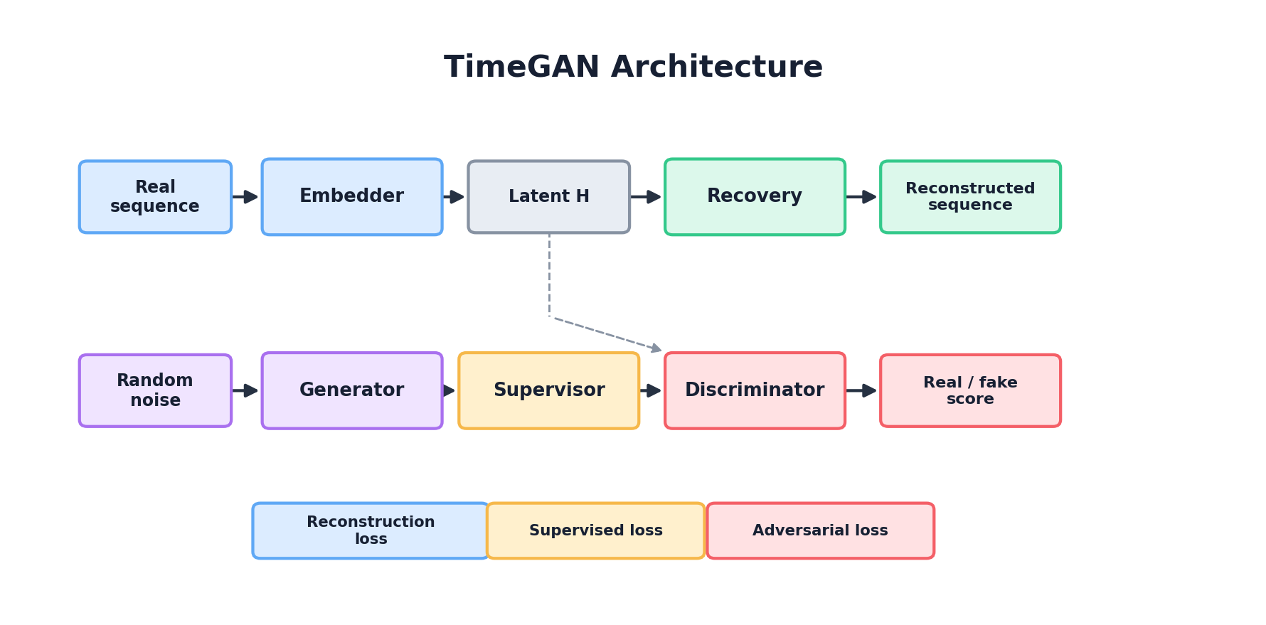
TimeGAN [6], introduced by Yoon, Jarrett, and van der Schaar at NeurIPS 2019, combines adversarial training with a supervised "reconstruction" loss in a learned embedding space. The key insight is that fooling a discriminator alone may not preserve temporal dynamics — a sequence could be adversarially convincing yet fail to honor lag-dependencies. TimeGAN adds an encoder-decoder pair that maps real sequences into a learned latent space, and a generator that produces latent-space sequences. An autoencoder loss forces the latent representations to be reconstructible, while an adversarial loss pushes generated sequences to be indistinguishable from real ones. The result is a model that learns both what values are plausible and how they should evolve.
In pseudocode:
# Simplified TimeGAN structure
class TimeGAN(nn.Module):
    def __init__(self, hidden_dim, seq_len, n_features):
        # Embedding: maps real/synthetic sequences to latent space
        self.embedding = RNNEncoder(seq_len, n_features, hidden_dim)

        # Generator: produces sequences in latent space
        self.generator = RNNGenerator(hidden_dim, seq_len, n_features)

        # Discriminator: judges realism in embedding space
        self.discriminator = RNNDiscriminator(hidden_dim, seq_len)

        # Recovery (reconstruction decoder)
        self.recovery = RNNDecoder(hidden_dim, seq_len, n_features)

    def forward(self, real_seq):
        # Encode real sequence
        embedded_real = self.embedding(real_seq)

        # Generate synthetic sequence in latent space
        noise = sample_noise(batch_size, hidden_dim)
        generated_latent = self.generator(noise)

        # Reconstruct synthetic sequence from latent
        synthetic_seq = self.recovery(generated_latent)

        # Discriminate real vs. generated in embedding space
        disc_real = self.discriminator(embedded_real)
        disc_fake = self.discriminator(generated_latent)

        # Compute losses
        adversarial_loss = bce_loss(disc_real, ones) + bce_loss(disc_fake, zeros)
        reconstruction_loss = mse_loss(real_seq, self.recovery(embedded_real))

        # Supervised loss: teacher-force the generator on the real embedded
        # sequence and ask it to predict the next-step embedding. This
        # directly pushes the generator to learn the step-to-step dynamics
        # of the real sequence in latent space.
        predicted_next = self.generator(embedded_real[:, :-1])
        supervised_loss = mse_loss(predicted_next, embedded_real[:, 1:])

        return adversarial_loss + reconstruction_loss + supervised_loss
Transformer-Based Generators
Transformers [7] excel at capturing long-range dependencies through self-attention. Unlike RNNs (which process sequences step-by-step) or CNNs (which have limited receptive fields), Transformers compute attention weights across the entire sequence, letting the model learn which past values are most relevant for predicting the future. For synthetic time-series generation, Transformer-based generators can be trained with a causal masking scheme: at position t, the model attends only to positions ≤ t. This naturally enforces autoregressive generation.
The trade-off is computational cost: Transformers scale as O(T²) in sequence length, which becomes prohibitive for very long sequences. But for moderate-length multivariate series with rich dependencies, they are state-of-the-art.
Temporal VAEs
Variational Autoencoders [8] can be extended to sequences by replacing standard fully-connected layers with RNNs or Transformers. A temporal VAE learns to map sequences to a latent normal distribution, then decode latent samples back into sequences. The ELBO (evidence lower bound) objective balances reconstruction (matching real sequences) against a KL regularization that keeps the latent distribution close to standard normal. This allows principled sampling: you can generate synthetic sequences by sampling from the latent prior and decoding.
Temporal VAEs offer interpretable latent spaces and can naturally handle variable-length sequences (via masking), but they often struggle with highly stochastic or multi-modal data — the KL term pushes the model toward a single "average" sequence, smoothing away diversity.
Diffusion Models for Time Series
Diffusion models [9] have recently emerged as a powerful alternative. They iteratively corrupt clean sequences by adding noise, then learn to reverse this process. For generation, you start with pure noise and denoise it, step by step, into a synthetic sequence. The key advantage is stability: diffusion avoids the mode-collapse and training instability of GANs. Recent models like TimeGrad [10] and CSDI [11] apply diffusion specifically to time-series forecasting and imputation, and the generative capability extends naturally to synthetic data.
Diffusion models are slower at inference (many denoising steps required) but often produce higher-quality, more diverse sequences than discriminative or VAE-based approaches.
Comparison Table
| Architecture | Strengths | Weaknesses | Best For |
|---|---|---|---|
| TimeGAN | Interpretable embedding; combines adversarial + supervised objectives | GAN training instability; limited to learned latent space | Multivariate medical, financial time series |
| Transformer-based | Long-range dependencies; parallelizable; flexible architectures | O(T²) complexity; requires careful masking | Long sequences; multi-modal dependencies |
| Temporal VAE | Stable training; interpretable latent; variable-length support | Mode-collapse toward average sequence; limited diversity | Well-structured, low-variance time series |
| Diffusion | Stable; high quality; rich diversity | Slow inference; many denoising steps required | High-quality synthesis when speed is secondary |
13.4 Sequence-Aware Evaluation
Evaluating a sequence generator is harder than evaluating a tabular generator. Standard fidelity metrics — Jensen-Shannon divergence, maximum mean discrepancy — compare marginal distributions. They are blind to temporal structure. A generator could produce synthetic sequences where every column matches the real data perfectly, yet the sequences are useless for forecasting because lag-dependencies are destroyed.
Why Standard Fidelity Metrics Break
Consider a simple example: a sequence of fair coin flips, where HEADS and TAILS each occur with probability 0.5 and successive flips are independent (so the true lag-1 autocorrelation is 0). A "bad" synthetic generator that produces HEADS, TAILS, HEADS, TAILS, HEADS, TAILS, ... matches the marginal distribution perfectly (50% heads, 50% tails) but has a lag-1 autocorrelation of −1 — every step deterministically flips the previous outcome. The synthetic sequence is wildly anti-correlated compared to the real one, yet any metric that looks only at the marginal would rate it excellent. A forecasting model trained on it would immediately fail on real data.
Temporal Fidelity Metrics
Good evaluation requires metrics that explicitly measure temporal structure:
- Autocorrelation preservation: Compare lag-k autocorrelation between real and synthetic for multiple lags (1, 7, 24, 52 depending on periodicity). The synthetic series should show similar decay patterns.
- Spectral density comparison: Compute the power spectral density (via FFT) for real and synthetic. Peaks reveal seasonality and dominant frequencies. Kullback-Leibler divergence or Wasserstein distance between spectral densities provides a scalar metric.
- First-difference distribution: For differenced series (period-over-period changes), compare marginal distributions. Preserves information about volatility and regime changes that point-wise measures miss.
- Dynamic Time Warping (DTW): Measures distance between sequences accounting for temporal shifts. Useful for checking that event ordering and transition patterns are preserved.
Train-on-Synthetic-Test-on-Real (TSTR)
The gold standard for evaluating synthetic time-series is the forecasting-oriented analogue of TSTR: train a forecasting model on synthetic sequences, evaluate on held-out real sequences, and compare to a model trained on real data. If synthetic → real forecasting performs nearly as well as real → real, the synthetic data captured the temporal structure needed for the task.
TimeGAN papers report two metrics in this vein [6]:
- Discriminative score: Train a GRU classifier on real sequences to predict a target variable (e.g., disease outcome). Measure the classifier's AUROC. Then train an identical classifier on synthetic sequences and evaluate on the real test set. The ratio (or difference) of AUROC values indicates whether synthetic sequences preserved predictive features.
- Predictive score: Use a GRU encoder-decoder as a sequence-to-sequence forecaster. Train on real, test on real. Then train on synthetic, test on real. Compare mean absolute error (MAE) or root mean squared error (RMSE) to see if the synthetic-trained forecaster generalizes.
Privacy Evaluation for Sequences
Sequential data poses unique privacy challenges. A single unique trajectory can be far more identifying than any individual row. Standard row-level membership inference attacks are insufficient. Instead, evaluate:
- Sequence-level nearest neighbors: For each synthetic sequence, find the closest real sequence (via DTW or Euclidean distance in a learned embedding). If synthetic sequences cluster tightly around real ones, privacy is at risk.
- Trajectory re-identification: In multi-entity datasets (e.g., many patients), can an adversary link a synthetic trajectory to a specific real individual? Measure this via a worst-case re-identification attack.
- Rare-event memorization: Do synthetic sequences reproduce rare events (equipment failures, fraud bursts, disease patterns) seen in the training data? Evaluate via frequency matching of outlier patterns.
13.5 Practical Patterns & Pitfalls
Moving from algorithm to practice, several design decisions and failure modes recur across projects.
Handling Irregular Timestamps & Missing Values
Not all sequences are regularly spaced. Event logs have gaps; sensor data may be missing for hours or days; transactional records arrive unpredictably. Before fitting a temporal generator:
- Decide representation: Do you encode missingness explicitly (a null value, a flag, or a masking token) or impute/interpolate first? Imputation smooths away information, but explicit missingness adds complexity.
- Handle irregular spacing: Some models (RNN-based) can use elapsed-time embeddings: encode the number of steps or hours since the last observation. Others require resampling to a fixed frequency (e.g., daily, hourly) with explicit handling of gaps.
- Preserve patterns in missingness: If missingness is informative (e.g., sensor offline means no measurement, which itself is a signal), encode it. A model that regenerates sequences with unrealistic missingness patterns will fail downstream.
Multivariate Generation & Cross-Series Dependence
Real-world sequences are often multivariate. A patient's vitals include heart rate, blood pressure, SpO2, and temperature. A factory's telemetry includes multiple sensors. Dependencies between variables matter: heart rate spikes together with blood pressure; temperature and humidity are correlated. A naive approach treats each variable independently, losing this coupling.
Better approaches jointly model multivariate series:
- Vector autoregressions (VAR): Extend ARIMA to multiple variables by modeling each as a linear combination of past values of all variables. Fast, interpretable, but limited to linear dynamics.
- Multivariate RNNs/Transformers: Process all variables together in each RNN cell or Transformer layer. Cross-variable attention learns which variables drive which. More expressive but requires careful regularization to avoid overfitting.
- Hierarchical or copula-based models: Model univariate marginals independently, then capture multivariate dependence via a copula [12]. Useful when dimensions are high and dependencies are not too exotic.
Conditioning on External Signals
Many real sequences are driven by external factors: energy consumption driven by weather and time-of-day; stock prices affected by macroeconomic news; patient trajectories influenced by treatments and diagnoses. Ignoring these signals, a generator may learn average dynamics but miss regime shifts.
To condition the generator:
- Exogenous variable embedding: If weather (temperature, humidity) drives power demand, include weather as a known exogenous input at every timestep. The RNN/Transformer conditions on this signal.
- Static attributes: Some conditioning is constant per sequence (patient age, machine model, geographic region). Embed these once and use them to initialize hidden states or modulate the network's behavior throughout.
- Control variates: If you want to generate sequences under specific scenarios (high vs. low demand, patient with vs. without comorbidity), use a classifier or regressor to predict which scenario a sequence falls into, then condition generation on that label.
Privacy Considerations: Trajectory De-anonymization
Temporal data raises privacy risks beyond traditional row-level concerns. A sequence is often much more identifying than any individual value. If a synthetic trajectory happens to match a real patient's heart-rate pattern over a 72-hour ICU stay, that patient is identified even if no explicit identifier is present.
Mitigations [13]:
- Differential privacy for sequences: Apply DP-SGD [14] during training, adding noise to gradients to guarantee formal privacy bounds. The cost is reduced utility, but the guarantee is provable.
- Sequence truncation: If full trajectories are identifying, release only short windows (e.g., 24 hours instead of 30 days). Shorter windows are harder to match to real individuals.
- Aggregation & smoothing: Before synthesis, aggregate across multiple entities (e.g., average multiple patient trajectories) or smooth with noise. You lose fine-grained dynamics but reduce re-identification risk.
- Empirical privacy auditing: For each synthetic sequence, compute its distance (in a learned embedding space) to the closest real sequence. If many synthetic sequences are very close to real ones, privacy risk is high.
13.6 Tools & Libraries
Rather than building from scratch, leverage existing ecosystems:
Gretel Synthetics (DoppelGANger / DGAN)
Gretel's DGAN implementation [15] is based on the DoppelGANger architecture (Lin et al., 2020), a GAN tailored for multivariate time series with both continuous and categorical attributes. It separates generation of time-invariant metadata from the temporal features and uses a conditional generation scheme to better preserve autocorrelation. Gretel ships it as part of a production-ready pipeline with integrated privacy tooling.
Synthetic Data Vault (SDV)
SDV is an open-source Python library (MIT licensed) specializing in synthetic tabular and relational data. Its sequential data module offers PARSynthesizer, a probabilistic autoregressive model that factorizes multivariate sequences and scales to moderate-length data. SDV also includes SDMetrics for evaluation, with sequence-aware metrics like InterRowMSAS [16].
Key SDV classes for time series:
from sdv.sequential import PARSynthesizer
from sdv.metadata import SingleTableMetadata

# Define metadata: identify sequence key and index columns
metadata = SingleTableMetadata()
metadata.add_column('patient_id', 'id')  # sequence key
metadata.add_column('time', 'datetime')  # sequence index
metadata.add_column('heart_rate', 'numerical')
metadata.add_column('blood_pressure', 'numerical')
metadata.set_sequence_key('patient_id')
metadata.set_sequence_index('time')

# Fit generator
synthesizer = PARSynthesizer(metadata)
synthesizer.fit(real_sequences)

# Generate synthetic sequences
synthetic_sequences = synthesizer.sample(num_sequences=100)

# Evaluate
from sdmetrics.sequential import evaluate
scores = evaluate(real_sequences, synthetic_sequences)
TSA (Time Series Augmentation) Libraries
For specific domains, specialized libraries exist. In healthcare, MITRE's Synthea [17] generates synthetic patient records including temporal trajectories. In finance, libraries like yfinance and zipline couple historical data retrieval with simulation. In manufacturing and IoT, custom simulators often outperform generic generators.
Research Implementations
TimeGAN, TimeGrad, and CSDI all have open-source reference implementations on GitHub. However, these are research-quality code and require careful tuning. Use them for experiments and prototyping, but rely on validated production libraries for production systems.
Choosing the Right Tool
| Use Case | Recommended Tool | Rationale |
|---|---|---|
| Tabular data with time columns | SDV (any synthesizer) | Flexible, open-source, well-documented |
| Regular multivariate time series, moderate length | SDV PARSynthesizer or TimeGAN | PAR is simple and fast; TimeGAN captures richer dynamics |
| Healthcare patient trajectories | Synthea or custom ARIMA/VAR + domain constraints | Synthea encodes medical logic; custom models ensure compliance |
| Financial or energy data, high stakes | Gretel DGAN or custom diffusion model | Production-ready privacy guarantees; diffusion for high quality |
| Research: exploring new architectures | PyTorch/TensorFlow + TimeGAN/TimeGrad reference code | Full control; understand the method end-to-end |
13.7 Summary & Key Takeaways
Sequential data is the frontier of synthetic data generation. It requires models that respect temporal dependence, not just marginal distributions. Classical approaches (ARIMA, HMMs, block bootstrap) remain invaluable for interpretability and speed. Deep generative models (TimeGAN, diffusion, Transformers) scale to complex, multivariate settings but demand careful evaluation.
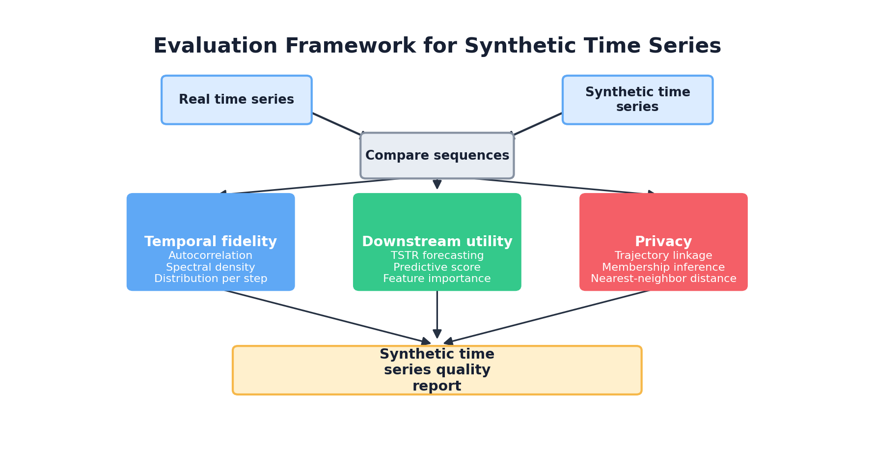
The evaluation framework for sequences is three-layered: (1) marginal fidelity, (2) temporal dynamics (autocorrelation, seasonality, spectral structure), and (3) downstream task utility (TSTR for forecasting or classification). Privacy evaluation must be sequence-aware, checking for trajectory-level re-identification risk.
Practical lessons:
- Start simple: Block bootstrap or ARIMA should beat your deep model, or your deep model is misconfigured.
- Represent sequences correctly: Use explicit sequence_key and sequence_index. Do not flatten temporal data into arbitrary tables.
- Handle conditioning: External signals (weather, treatments, news) drive real sequences. Condition your generator explicitly.
- Audit privacy at the sequence level: Check nearest-neighbor distances and re-identification risk by trajectory, not by row.
- Validate on downstream tasks: TSTR is not optional. Train a forecaster on synthetic, test on real, and compare to baseline.
Academic References
- (2019). Modeling Tabular Data using Conditional GAN. Advances in Neural Information Processing Systems (NeurIPS). arxiv.org/abs/1907.00503
- (1976). Time Series Analysis: Forecasting and Control. Revised Edition. Holden-Day.
- (2012). Time Series Analysis by State Space Methods. Oxford University Press, 2nd Edition.
- (1989). The Jackknife and the Bootstrap for General Stationary Observations. Annals of Statistics, 17(3), 1217–1241.
- (1966). Statistical Inference for Probabilistic Functions of Finite State Markov Chains. Journal of the Mathematical Analysis and Applications, 12(2), 200–210.
- (2019). Time-series Generative Adversarial Networks. Advances in Neural Information Processing Systems (NeurIPS). papers.nips.cc
- (2017). Attention Is All You Need. Advances in Neural Information Processing Systems (NeurIPS). arxiv.org/abs/1706.03762
- (2014). Auto-Encoding Variational Bayes. International Conference on Learning Representations (ICLR). arxiv.org/abs/1312.6114
- (2020). Denoising Diffusion Probabilistic Models. Advances in Neural Information Processing Systems (NeurIPS). arxiv.org/abs/2006.11239
- (2021). Autoregressive Denoising Diffusion Models for Multivariate Probabilistic Time Series Forecasting. International Conference on Machine Learning (ICML). proceedings.mlr.press/v139/rasul21a.html
- (2021). Csdi: Conditional Score-based Diffusion Models for Probabilistic Time Series Imputation. Advances in Neural Information Processing Systems (NeurIPS). arxiv.org/abs/2107.03502
- (2006). An Introduction to Copulas. Springer, 2nd Edition.
- (2020). Practical Synthetic Data Generation: Balancing Privacy and the Broad Availability of Data. O'Reilly Media.
- (2016). Deep Learning with Differential Privacy. ACM Conference on Computer and Communications Security (CCS). arxiv.org/abs/1607.00133
- (2020). Using GANs for Sharing Networked Time Series Data: Challenges, Initial Promise, and Open Questions (DoppelGANger). ACM Internet Measurement Conference (IMC). arxiv.org/abs/1909.13403
- (2023). SDMetrics: Metrics for Evaluating Synthetic Data. Open-source Python library. github.com/sdv-dev/SDMetrics
- (2018). Synthea: An Approach, Method, and Software Mechanism for Generating Synthetic Patients and the Synthetic Electronic Health Care Record. Journal of the American Medical Informatics Association, 25(3), 230–238. academic.oup.com/jamia/article/25/3/230