Chapter 9: Evaluation & Quality Metrics

9.1 Why Evaluation Matters

You have generated synthetic data. The generator ran without errors, sampled thousands of records, and the output looks plausible at first glance. But can you trust it?

The answer depends entirely on rigorous evaluation. Synthetic data quality is not self-evident. A GAN trained on financial transactions might produce structurally sound records that violate statistical invariants. A VAE fine-tuned on medical data might capture marginal distributions but fail to preserve disease correlations. A rule-based simulator might be reproducible and auditable but generate such narrow distribution support that it has limited utility for model training.

Evaluation is the bridge between generation and deployment. It answers the critical question: does this synthetic data actually serve the purpose for which it was created? Without systematic evaluation, you risk deploying synthetic data that appears to work but silently undermines downstream decisions, or that reveals more about real data than you realized.

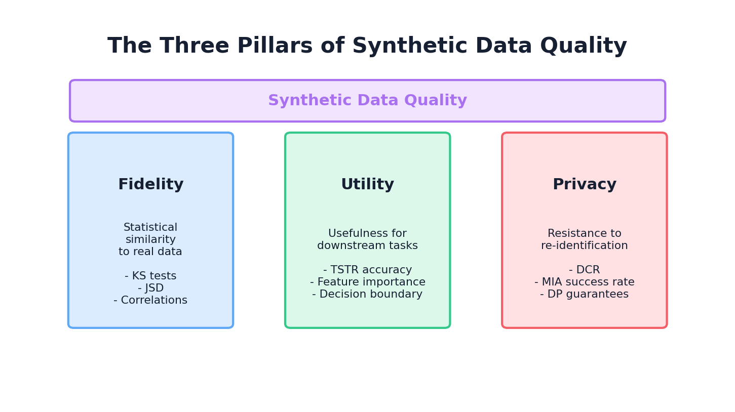
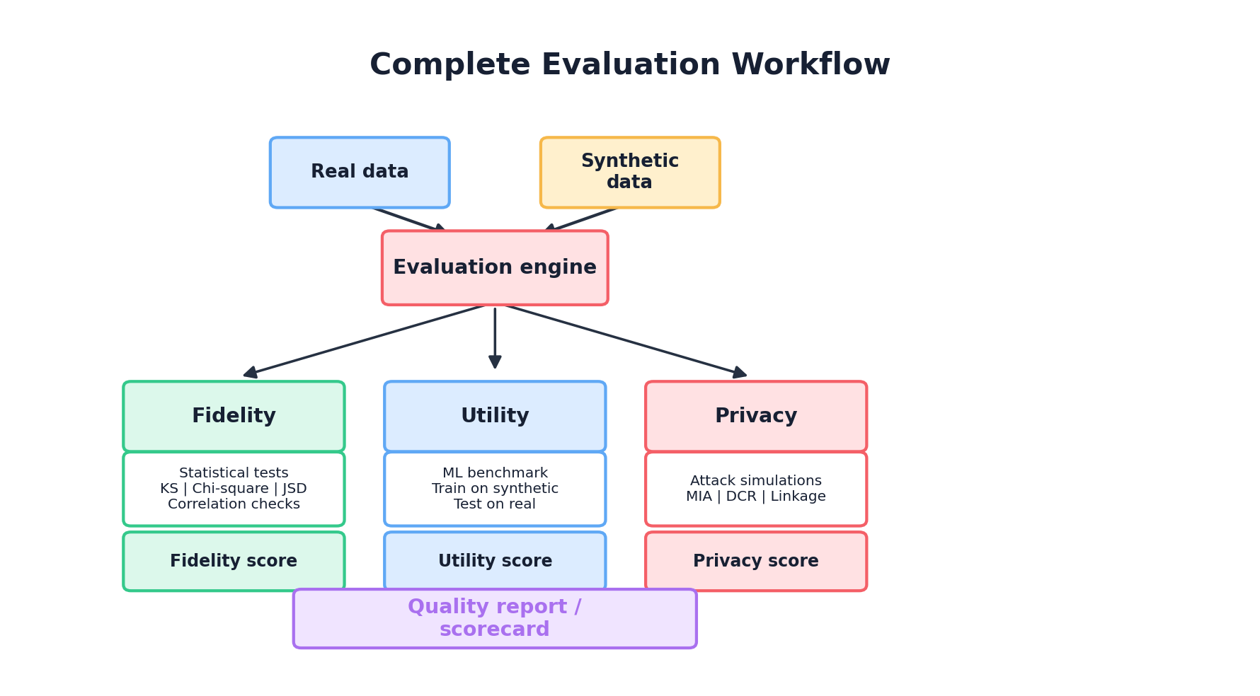
This chapter provides a complete framework for evaluating synthetic data across three complementary dimensions: fidelity (how similar is the synthetic data to the real data?), utility (how useful is it for downstream tasks?), and privacy (how well are real individuals protected?). We'll move from theory to implementation, showing how to compute metrics, interpret them, and build automated evaluation pipelines.

9.2 The Three Pillars of Synthetic Data Quality

Synthetic data quality rests on three foundational pillars, each answering a different question:

Pillar 1: Fidelity

The Question: How well does the synthetic data resemble the real data in terms of statistical properties?

Fidelity measures the degree to which synthetic data preserves the statistical characteristics of the real data. This includes univariate distributions (marginals), bivariate and multivariate relationships, temporal patterns, and structural constraints. High fidelity means that if you analyze the synthetic data, you observe similar statistical conclusions as you would from the real data.

Why it matters: If synthetic data has poor fidelity, it cannot serve as a drop-in replacement for real data. Statistical analyses will be misleading, regression coefficients will be biased, and domain-specific patterns will be lost. Fidelity is the floor—without it, nothing else matters.

Example: A synthetic dataset is created to simulate patient demographics. Real data shows that age is normally distributed with mean 55 and std 18, and that older patients have higher hypertension prevalence (70% at age 70+, 30% at age 40-50). If synthetic age is uniformly distributed or the age-hypertension correlation is absent, fidelity is compromised.

Pillar 2: Utility

The Question: How well does the synthetic data enable downstream machine learning tasks?

Utility measures whether models trained on synthetic data generalize to real data, and whether insights derived from synthetic data are actionable on real data. A dataset can have perfect fidelity in marginal distributions but fail utility if it lacks important interaction effects or rare subgroups that are critical for model performance.

Why it matters: The ultimate purpose of synthetic data is often to train models or support analysis. If a model trained on synthetic data fails to generalize to real data, or if analysis conclusions don't hold, synthetic data has failed its primary mission regardless of how statistically perfect it appears.

Example: A synthetic loan dataset has perfect correlation structure but is missing the rare "defaulting subprime borrower" subgroup that dominates risk in the real loan book. A classifier trained on synthetic data will overestimate precision and miss true default cases in production.

Pillar 3: Privacy

The Question: How well are real individuals protected from re-identification and attribute inference?

Privacy measures the extent to which synthetic data leaks information about real individuals. This is particularly critical when synthetic data is shared externally or used for collaborative research. Privacy attacks (membership inference, attribute inference, linkage) can succeed even if synthetic data has high fidelity.

Why it matters: Privacy breaches can expose individuals, violate regulations (GDPR, HIPAA), destroy trust, and create legal liability. Synthetic data that is utility-rich but privacy-poor is worse than useless—it's dangerous. Privacy must be assessed alongside fidelity and utility.

Example: A synthetic medical dataset reproduces disease prevalences and comorbidities perfectly but, when combined with zip code and age, uniquely identifies individuals in the real cohort through linkage attack. High fidelity and utility do not compensate for failed privacy.

9.3 Statistical Fidelity Metrics

Fidelity metrics quantify how closely synthetic data mirrors the statistical properties of real data. We begin with univariate (column-wise) metrics, then move to bivariate and multivariate comparisons.

9.3.1 Univariate Metrics: Kolmogorov-Smirnov Test

The Kolmogorov-Smirnov (KS) test measures the maximum distance between the empirical cumulative distribution functions (CDFs) of real and synthetic data for a continuous variable.

Interpretation: KS statistic ranges from 0 (identical distributions) to 1 (maximally different). An 0.05 p-value indicates significant difference at the 5% level. A small KS statistic (e.g., 0.02) suggests good univariate fidelity.

Limitation: KS test is sensitive to sample size. With large samples, even tiny practical differences become significant. It also doesn't capture multivariate structure.

9.3.2 Univariate Metrics: Chi-Square Test

For categorical variables, the chi-square test compares observed vs. expected frequencies across categories.

Formula: χ² = Σ((observed - expected)² / expected)

Interpretation: A small chi-square statistic and high p-value indicate that categorical distributions are not distinguishable by this test. Treat 0.05 as a conventional screening threshold, not a proof that the distributions are the same.

9.3.3 Univariate Metrics: Jensen-Shannon Divergence

Jensen-Shannon (JS) divergence is a symmetrised version of Kullback-Leibler divergence between two probability distributions. It is well-defined when the supports overlap imperfectly (the KL divergence blows up in that case), making it a common fidelity metric for discrete or binned distributions.

Formula: JS(P ∥ Q) = 0.5 · KL(P ∥ M) + 0.5 · KL(Q ∥ M), where M = 0.5 · (P + Q).

Units and range. With natural log, JS divergence ∈ [0, ln 2] ≈ [0, 0.693]; with log base 2, JS divergence ∈ [0, 1]. Note that scipy.spatial.distance.jensenshannon returns the Jensen-Shannon distance (the square root of the divergence), not the divergence itself, so its values lie in [0, √ln 2] ≈ [0, 0.832] by default — or [0, 1] when base=2 is passed. The code below is consistent with the distance convention; square the result if you want the divergence in nats (or pass base=2 for bits).

Code: Computing Univariate Metrics

import pandas as pd
import numpy as np
from scipy.stats import ks_2samp, chi2_contingency
from scipy.spatial.distance import jensenshannon

def compute_univariate_fidelity(real_df, synthetic_df):
    """
    Compute KS, chi-square, and JS divergence for all columns.

    Args:
        real_df: Real data (pd.DataFrame)
        synthetic_df: Synthetic data (pd.DataFrame)

    Returns:
        dict: Metrics per column
    """
    results = {}

    for col in real_df.columns:
        real_col = real_df[col].dropna()
        synth_col = synthetic_df[col].dropna()

        if real_col.dtype in ['int64', 'float64']:
            # Continuous: KS test
            ks_stat, ks_pval = ks_2samp(real_col, synth_col)
            results[col] = {
                'type': 'continuous',
                'ks_stat': ks_stat,
                'ks_pval': ks_pval,
            }

            # JS divergence (with histogram binning)
            bins = min(50, int(np.sqrt(len(real_col))))
            hist_real, bin_edges = np.histogram(real_col, bins=bins, density=True)
            hist_synth, _ = np.histogram(synth_col, bins=bin_edges, density=True)
            # Normalize
            hist_real = hist_real / hist_real.sum()
            hist_synth = hist_synth / hist_synth.sum()
            # scipy returns the JS *distance*; square it for the divergence in nats.
            js_distance = jensenshannon(hist_real, hist_synth)
            results[col]['js_distance'] = js_distance
            results[col]['js_divergence_nats'] = js_distance ** 2
        else:
            # Categorical: chi-square test
            real_counts = real_col.value_counts()
            synth_counts = synth_col.value_counts()

            # Align categories
            all_cats = set(real_counts.index) | set(synth_counts.index)
            real_counts = real_counts.reindex(all_cats, fill_value=0)
            synth_counts = synth_counts.reindex(all_cats, fill_value=0)

            # Create contingency table
            contingency = np.array([real_counts.values, synth_counts.values])
            chi2, pval, dof, expected = chi2_contingency(contingency)

            results[col] = {
                'type': 'categorical',
                'chi2_stat': chi2,
                'chi2_pval': pval,
                'categories': len(all_cats),
            }

    return results

# Example usage
real_data = pd.read_csv('real_patients.csv')
synthetic_data = pd.read_csv('synthetic_patients.csv')

fidelity_metrics = compute_univariate_fidelity(real_data, synthetic_data)

# Print summary
print("\\n=== Univariate Fidelity Metrics ===")
for col, metrics in fidelity_metrics.items():
    if metrics['type'] == 'continuous':
        print(f"{col}: KS={metrics['ks_stat']:.4f} (p={metrics['ks_pval']:.4f}), "
              f"JS_dist={metrics['js_distance']:.4f}")
    else:
        print(f"{col}: χ²={metrics['chi2_stat']:.2f} (p={metrics['chi2_pval']:.4f})")
      

9.3.4 Multivariate Fidelity: Propensity-Score MSE (pMSE)

Per-column KS and JS scores can all look great while the joint distribution is badly distorted. A widely used multivariate fidelity summary is the propensity-score MSE (pMSE) of Woo et al. (2009). Pool real and synthetic rows, label them 0 and 1, fit a classifier (logistic regression or gradient boosting) to tell them apart, and record how close its predicted probabilities stay to 0.5.

Formula: pMSE = (1/N) · Σᵢ (p̂ᵢ − c)², where p̂ᵢ is the classifier's estimated probability that row i is synthetic, c = N_synth / N is the class balance, and N is the total pool size. A perfect generator gives p̂ᵢ ≈ c for every row and pMSE → 0; an easily distinguishable one drives pMSE up toward c(1 − c).

from sklearn.linear_model import LogisticRegression
from sklearn.model_selection import cross_val_predict

def pmse(real_df, synth_df, numeric_only=True, seed=0):
    """Propensity-score MSE (Woo et al., 2009). Lower is better; 0 = perfect."""
    if numeric_only:
        real_df = real_df.select_dtypes(include=[np.number])
        synth_df = synth_df.select_dtypes(include=[np.number])
    X = np.vstack([real_df.values, synth_df.values])
    y = np.concatenate([np.zeros(len(real_df)), np.ones(len(synth_df))])
    c = y.mean()  # fraction of synthetic rows in the pool

    # Use out-of-fold probabilities so we don't grade the classifier on training data.
    probs = cross_val_predict(
        LogisticRegression(max_iter=1000, random_state=seed),
        X, y, cv=5, method='predict_proba',
    )[:, 1]
    return float(np.mean((probs - c) ** 2))

print(f"pMSE: {pmse(real_data, synthetic_data):.5f}")
      

Interpretation: pMSE is model-dependent. A flexible classifier (gradient boosting) gives a stricter test than logistic regression, so always report which model you used alongside the score.

9.3.5 Pairwise Metrics: Correlation Matrix Comparison

Univariate metrics miss multivariate structure. A key relationship is the correlation between variables. Comparing correlation matrices between real and synthetic data reveals whether the generator preserved pairwise dependencies.

Approach: Compute Pearson or Spearman correlation matrices for both datasets, then measure distance between them using Frobenius norm or sum of absolute differences.

Metric: Correlation difference = ||R_real - R_synthetic||_F / ||R_real||_F

Values close to 0 indicate preserved correlations. Values > 0.1 suggest significant structural differences.

Code: Correlation Matrix Comparison

from scipy.spatial.distance import euclidean

def compare_correlation_matrices(real_df, synthetic_df):
    """
    Compare correlation matrices between real and synthetic data.
    """
    # Select numeric columns only
    numeric_real = real_df.select_dtypes(include=[np.number])
    numeric_synth = synthetic_df.select_dtypes(include=[np.number])

    # Compute correlation matrices
    corr_real = numeric_real.corr()
    corr_synth = numeric_synth.corr()

    # Frobenius norm (matrix distance)
    diff_norm = np.linalg.norm(corr_real.values - corr_synth.values, 'fro')
    real_norm = np.linalg.norm(corr_real.values, 'fro')
    normalized_diff = diff_norm / real_norm if real_norm > 0 else 0

    # Per-pair absolute differences
    corr_diff = (corr_real - corr_synth).abs()
    max_pair_diff = corr_diff.values[np.triu_indices_from(
        corr_diff.values, k=1)].max()
    mean_pair_diff = corr_diff.values[np.triu_indices_from(
        corr_diff.values, k=1)].mean()

    return {
        'frobenius_norm_diff': diff_norm,
        'normalized_frobenius_diff': normalized_diff,
        'max_pair_difference': max_pair_diff,
        'mean_pair_difference': mean_pair_diff,
        'corr_real': corr_real,
        'corr_synth': corr_synth,
    }

# Example
corr_comparison = compare_correlation_matrices(real_data, synthetic_data)
print(f"Normalized Correlation Difference: {corr_comparison['normalized_frobenius_diff']:.4f}")
print(f"Max Pairwise Correlation Diff: {corr_comparison['max_pair_difference']:.4f}")
      

9.4 Distribution Comparison Techniques

Beyond point-estimate tests, visual and quantitative distribution comparisons provide deeper insight into fidelity.

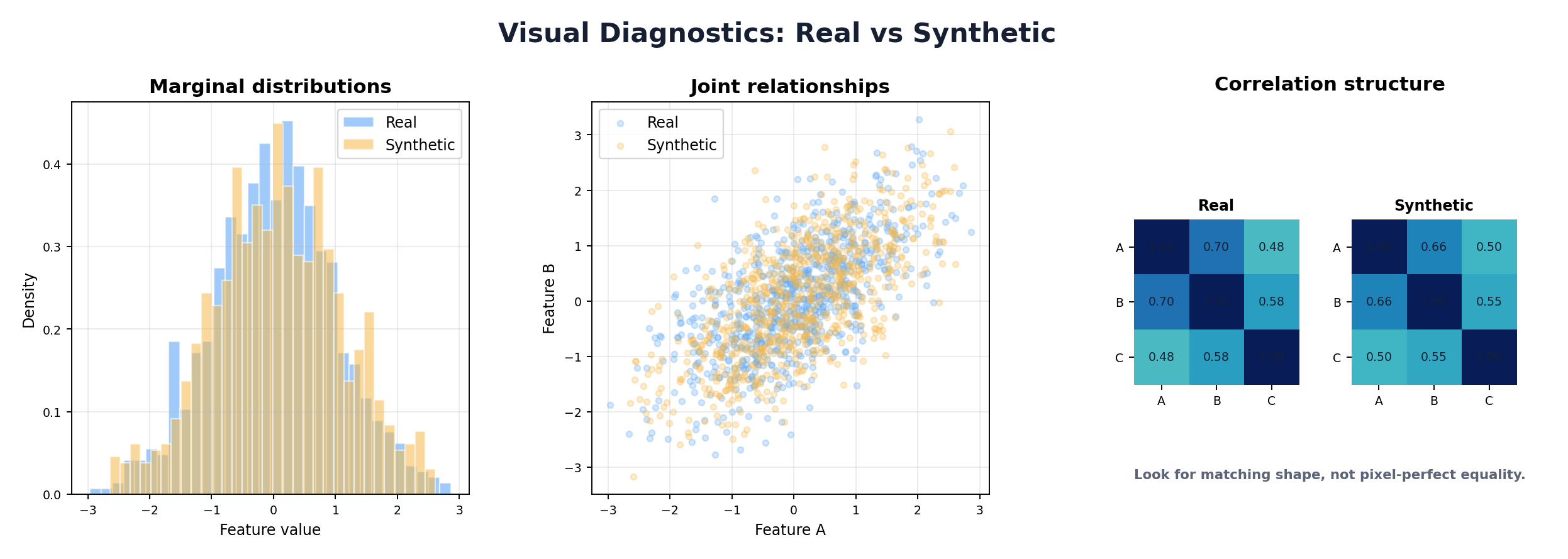
9.4.1 QQ Plots and Marginal Overlap

A QQ (quantile-quantile) plot compares quantiles of two distributions. If both distributions are identical, the QQ plot lies on the diagonal y=x. Deviations indicate distributional differences.

Interpretation: Points below the diagonal indicate that synthetic quantiles are lower than real quantiles at corresponding probability levels. This reveals where distributions diverge (tails vs. center).

Complementary approach: overlay histograms or kernel density estimates (KDE) of real and synthetic data. Areas of non-overlap highlight regions where the generator failed.

9.4.2 Earth Mover's Distance (Wasserstein Distance)

Earth Mover's Distance (EMD), also called Wasserstein distance, is the minimum cost to transport one distribution to another. For one-dimensional continuous data, it equals the area between the two CDFs.

Advantage: EMD is a true metric (satisfies triangle inequality), interpretable in the original data units, and sensitive to distributional shifts across all regions.

Interpretation: EMD of 0 = identical distributions. EMD = range of data / 100 is a rough threshold for "good" fidelity, though domain context matters.

Code: EMD and Distribution Plots

from scipy.stats import wasserstein_distance
import matplotlib.pyplot as plt

def compute_emd_and_plot(real_col, synth_col, column_name):
    """
    Compute Earth Mover's Distance and visualize distributions.
    """
    emd = wasserstein_distance(real_col.dropna(), synth_col.dropna())

    fig, axes = plt.subplots(1, 2, figsize=(12, 4))

    # Histogram + KDE
    ax = axes[0]
    ax.hist(real_col, bins=30, alpha=0.6, label='Real', density=True, color='blue')
    ax.hist(synth_col, bins=30, alpha=0.6, label='Synthetic', density=True, color='orange')
    ax.set_xlabel(column_name)
    ax.set_ylabel('Density')
    ax.legend()
    ax.set_title(f'{column_name} Distribution (EMD={emd:.4f})')

    # QQ Plot
    ax = axes[1]
    from scipy.stats import probplot
    probplot(synth_col.dropna(), dist="norm", plot=ax)
    ax.get_lines()[0].set_color('orange')
    ax.set_title(f'QQ Plot: {column_name}')

    plt.tight_layout()
    return emd, fig

# Compute EMD for all numeric columns
numeric_cols = real_data.select_dtypes(include=[np.number]).columns
emd_results = {}
for col in numeric_cols:
    emd, fig = compute_emd_and_plot(real_data[col], synthetic_data[col], col)
    emd_results[col] = emd
    plt.savefig(f'emd_{col}.png')
    plt.close()

print("Earth Mover's Distance per column:")
for col, emd in emd_results.items():
    print(f"  {col}: {emd:.4f}")
      

9.5 Machine Learning Utility Evaluation

The ultimate test of synthetic data is its utility for machine learning tasks. High fidelity is necessary but not sufficient—synthetic data must enable models to generalize to real data.

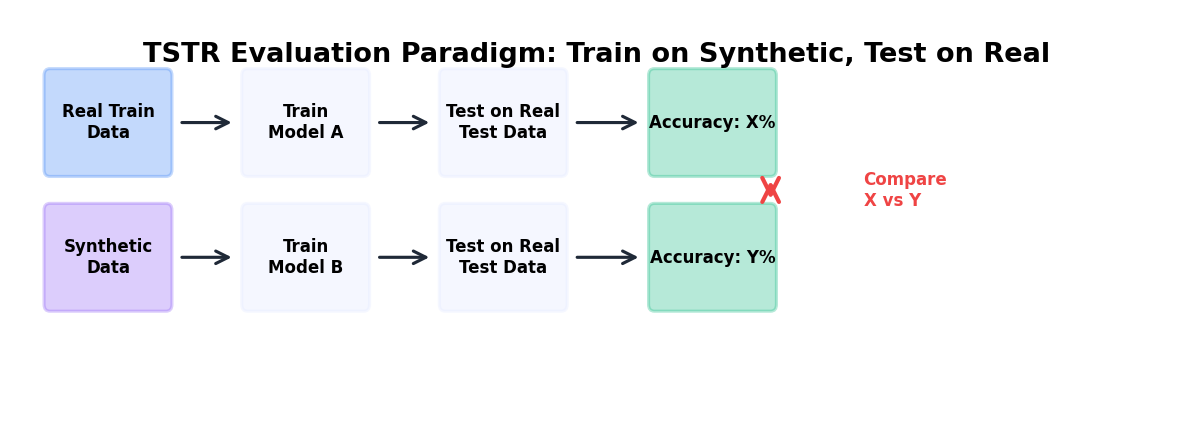
9.5.1 Train-on-Synthetic, Test-on-Real (TSTR)

TSTR is the canonical utility paradigm: train a model on synthetic data, evaluate it on real data (held-out test set). Compare TSTR performance to the baseline (train-on-real, test-on-real, TRTR).

Interpretation: If TSTR accuracy is within 5% of TRTR, synthetic data has good utility. Larger gaps (>10%) suggest that the synthetic data is missing patterns critical for the downstream task.

Why this works: TSTR directly measures whether a model trained on synthetic data can generalize to real data, the actual use case for synthetic data in production.

9.5.2 Reverse Scenario: Train-on-Real, Test-on-Synthetic (TRTS)

TRTS trains on real data and tests on synthetic data. If TRTS performance is significantly lower than TRTR, the synthetic distribution has shifted outside the decision boundaries learned by the model. This flags utility problems.

Use case: TRTS is useful for detecting when synthetic data is too different from real data despite good univariate fidelity (e.g., data with shifted correlations or rare subgroup omissions).

9.5.3 Feature Importance Comparison

Train models on both real and synthetic data, extract feature importances, and compare. If feature rankings differ significantly, the synthetic data is teaching the model different decision rules.

Metric: Spearman rank correlation of feature importances, or sum of absolute rank differences. Values close to 1 (or small rank differences) indicate consistency.

Code: Complete ML Utility Pipeline

from sklearn.model_selection import train_test_split
from sklearn.preprocessing import StandardScaler
from sklearn.ensemble import RandomForestClassifier
from sklearn.linear_model import LogisticRegression
from sklearn.metrics import accuracy_score, precision_score, recall_score, f1_score
import scipy.stats as stats

class MLUtilityEvaluator:
    """
    Comprehensive ML utility evaluation for synthetic data.
    Implements TSTR, TRTS, and feature importance comparison.
    """

    def __init__(self, real_df, synthetic_df, target_col, test_size=0.2, random_state=42):
        self.real_df = real_df
        self.synthetic_df = synthetic_df
        self.target_col = target_col
        self.test_size = test_size
        self.random_state = random_state
        self.results = {}

    def prepare_data(self, df):
        """Separate features and target, handle categorical variables."""
        X = df.drop(columns=[self.target_col])
        y = df[self.target_col]

        # One-hot encode categorical variables
        X = pd.get_dummies(X, drop_first=True)

        return X, y

    def train_and_evaluate(self, X_train, y_train, X_test, y_test, model_name='RF'):
        """Train a model and compute metrics."""
        if model_name == 'RF':
            model = RandomForestClassifier(n_estimators=100, random_state=self.random_state)
        elif model_name == 'LR':
            model = LogisticRegression(max_iter=1000)

        model.fit(X_train, y_train)
        y_pred = model.predict(X_test)

        metrics = {
            'accuracy': accuracy_score(y_test, y_pred),
            'precision': precision_score(y_test, y_pred, average='binary', zero_division=0),
            'recall': recall_score(y_test, y_pred, average='binary', zero_division=0),
            'f1': f1_score(y_test, y_pred, average='binary', zero_division=0),
        }

        return model, metrics

    def run_tstr(self, model_name='RF'):
        """Train on Synthetic, Test on Real (TSTR)."""
        X_real, y_real = self.prepare_data(self.real_df)
        X_synth, y_synth = self.prepare_data(self.synthetic_df)

        # Align feature columns
        common_cols = X_real.columns.intersection(X_synth.columns)
        X_real = X_real[common_cols]
        X_synth = X_synth[common_cols]

        X_real_train, X_real_test, y_real_train, y_real_test = train_test_split(
            X_real, y_real, test_size=self.test_size, random_state=self.random_state
        )

        # Train on synthetic (full set), test on real test set
        model, metrics = self.train_and_evaluate(
            X_synth, y_synth, X_real_test, y_real_test, model_name
        )

        self.results['TSTR'] = metrics
        self.results['TSTR_model'] = model
        return metrics

    def run_trtr(self, model_name='RF'):
        """Train on Real, Test on Real (TRTR) - baseline."""
        X_real, y_real = self.prepare_data(self.real_df)

        X_train, X_test, y_train, y_test = train_test_split(
            X_real, y_real, test_size=self.test_size, random_state=self.random_state
        )

        model, metrics = self.train_and_evaluate(
            X_train, y_train, X_test, y_test, model_name
        )

        self.results['TRTR'] = metrics
        self.results['TRTR_model'] = model
        return metrics

    def run_trts(self, model_name='RF'):
        """Train on Real, Test on Synthetic (TRTS)."""
        X_real, y_real = self.prepare_data(self.real_df)
        X_synth, y_synth = self.prepare_data(self.synthetic_df)

        # Align feature columns
        common_cols = X_real.columns.intersection(X_synth.columns)
        X_real = X_real[common_cols]
        X_synth = X_synth[common_cols]

        X_real_train, _, y_real_train, _ = train_test_split(
            X_real, y_real, test_size=self.test_size, random_state=self.random_state
        )

        model, metrics = self.train_and_evaluate(
            X_real_train, y_real_train, X_synth, y_synth, model_name
        )

        self.results['TRTS'] = metrics
        self.results['TRTS_model'] = model
        return metrics

    def compare_feature_importance(self):
        """Compare feature importances from TRTR vs TSTR models."""
        trtr_model = self.results.get('TRTR_model')
        tstr_model = self.results.get('TSTR_model')

        if trtr_model is None or tstr_model is None:
            return None

        # Extract feature importances
        X_real, _ = self.prepare_data(self.real_df)
        X_synth, _ = self.prepare_data(self.synthetic_df)
        common_cols = X_real.columns.intersection(X_synth.columns)

        if not hasattr(trtr_model, 'feature_importances_'):
            return None  # Not applicable to LR

        fi_trtr = trtr_model.feature_importances_
        fi_tstr = tstr_model.feature_importances_

        # Rank and compare
        rank_trtr = stats.rankdata(fi_trtr)
        rank_tstr = stats.rankdata(fi_tstr)

        rank_corr, rank_pval = stats.spearmanr(rank_trtr, rank_tstr)

        return {
            'spearman_rank_corr': rank_corr,
            'rank_pval': rank_pval,
            'feature_importances_trtr': fi_trtr,
            'feature_importances_tstr': fi_tstr,
            'features': list(common_cols),
        }

    def summary(self):
        """Print a summary report of utility evaluation."""
        print("\\n=== ML Utility Evaluation Report ===")
        print("\\nTRTR (Real→Real, Baseline):")
        for metric, value in self.results.get('TRTR', {}).items():
            print(f"  {metric}: {value:.4f}")

        print("\\nTSTR (Synthetic→Real):")
        for metric, value in self.results.get('TSTR', {}).items():
            print(f"  {metric}: {value:.4f}")

        if 'TSTR' in self.results and 'TRTR' in self.results:
            print("\\nTSTR vs TRTR Performance Gap (%):")
            for metric in ['accuracy', 'f1']:
                gap = (self.results['TRTR'][metric] -
                       self.results['TSTR'][metric]) * 100
                print(f"  {metric}: {gap:.2f}%")

        print("\\nTRTS (Real→Synthetic):")
        for metric, value in self.results.get('TRTS', {}).items():
            print(f"  {metric}: {value:.4f}")

        fi_comparison = self.compare_feature_importance()
        if fi_comparison:
            print(f"\\nFeature Importance Rank Correlation: {fi_comparison['spearman_rank_corr']:.4f}")

# Example usage
evaluator = MLUtilityEvaluator(
    real_data, synthetic_data, target_col='diagnosis', random_state=42
)

evaluator.run_trtr(model_name='RF')
evaluator.run_tstr(model_name='RF')
evaluator.run_trts(model_name='RF')
evaluator.summary()
      

9.6 Privacy Metrics and Attacks

Privacy evaluation is distinct from fidelity and utility. Even synthetic data with perfect fidelity can leak sensitive information. Privacy must be actively measured through attack simulations.

9.6.1 Distance to Closest Record (DCR)

DCR measures the minimum distance from each real record to any synthetic record in the feature space. If a real record is very close to a synthetic record, the synthetic record may be a near-copy or reconstruction of the real record.

Interpretation: Small DCR values (< 10th percentile of inter-record distances) suggest potential privacy leakage. The proportion of real records with DCR below a threshold indicates re-identification risk.

Typical threshold: If >5% of real records have DCR in the bottom 10th percentile of synthetic-to-synthetic distances, privacy may be compromised.

9.6.2 Membership Inference Attack (MIA)

A membership inference attack attempts to determine whether a specific record was in the training data. The attacker trains a classifier to predict "member" vs. "non-member" based on properties of the generator or synthetic data.

Simple approach: For each real record, compute its likelihood under the synthetic data distribution (e.g., kernel density estimate). Members of the training set often have higher likelihood. If the attacker can separate real training records from non-members by likelihood alone, membership is inferable.

Metric: MIA accuracy = accuracy of a classifier predicting membership given likelihood. Values near 50% indicate robustness (no signal); values > 60% indicate privacy leakage.

Code: Privacy Metrics

from scipy.spatial.distance import cdist
from sklearn.neighbors import KernelDensity
from sklearn.metrics import accuracy_score, roc_auc_score

def compute_dcr(real_df, synthetic_df, exclude_cols=None):
    """
    Compute Distance to Closest Record (DCR).
    """
    if exclude_cols is None:
        exclude_cols = []

    # Numeric columns only
    numeric_cols = [c for c in real_df.columns
                    if c not in exclude_cols and real_df[c].dtype in ['int64', 'float64']]

    real_num = real_df[numeric_cols].fillna(0).values
    synth_num = synthetic_df[numeric_cols].fillna(0).values

    # Normalize to [0,1]
    from sklearn.preprocessing import MinMaxScaler
    scaler = MinMaxScaler()
    real_num = scaler.fit_transform(real_num)
    synth_num = scaler.transform(synth_num)

    # Compute distances: each real record to closest synthetic record
    distances = cdist(real_num, synth_num, metric='euclidean')
    dcr = distances.min(axis=1)

    # Compute baseline: distance between random synthetic records
    synth_distances = cdist(synth_num, synth_num, metric='euclidean')
    np.fill_diagonal(synth_distances, np.inf)  # Exclude self-distance
    baseline_dcr_percentiles = synth_distances.min(axis=1)

    threshold_10pct = np.percentile(baseline_dcr_percentiles, 10)
    leak_ratio = (dcr < threshold_10pct).sum() / len(dcr)

    return {
        'dcr': dcr,
        'mean_dcr': dcr.mean(),
        'min_dcr': dcr.min(),
        'percentile_10_dcr': np.percentile(dcr, 10),
        'leak_ratio': leak_ratio,
        'baseline_threshold': threshold_10pct,
    }

def membership_inference_attack(members_df, non_members_df, synthetic_df,
                                exclude_cols=None):
    """
    Likelihood-based membership inference attack.

    Args
    ----
    members_df:     real records that WERE seen by the generator during fitting.
    non_members_df: real records that were HELD OUT from the generator.
    synthetic_df:   synthetic records produced by the generator.

    The attack assumes that, if the generator leaks, training members will sit
    in higher-density regions of the synthetic distribution than held-out
    records. We fit a KDE on the synthetic data and use its log-likelihood as
    the attacker's score; AUC measurably above 0.5 signals leakage.
    """
    if exclude_cols is None:
        exclude_cols = []

    numeric_cols = [c for c in members_df.columns
                    if c not in exclude_cols
                    and members_df[c].dtype in ['int64', 'float64']]

    M = members_df[numeric_cols].fillna(0).values
    N = non_members_df[numeric_cols].fillna(0).values
    S = synthetic_df[numeric_cols].fillna(0).values

    # Fit scaler on synthetic data so the attack does not peek at real data.
    from sklearn.preprocessing import StandardScaler
    scaler = StandardScaler().fit(S)
    M, N, S = scaler.transform(M), scaler.transform(N), scaler.transform(S)

    kde = KernelDensity(bandwidth=0.5).fit(S)
    ll_members = kde.score_samples(M)
    ll_non_members = kde.score_samples(N)

    scores = np.concatenate([ll_members, ll_non_members])
    y_true = np.concatenate([np.ones(len(ll_members)),
                             np.zeros(len(ll_non_members))])

    # Choose the threshold on a separate, random split to avoid using the
    # label to pick the cutoff we then report accuracy against.
    threshold = np.median(scores)
    y_pred = (scores > threshold).astype(int)

    mia_acc = accuracy_score(y_true, y_pred)
    try:
        mia_auc = roc_auc_score(y_true, scores)
    except ValueError:
        mia_auc = None

    return {
        'mia_accuracy': mia_acc,   # 0.5 = perfect privacy, > 0.6 = leakage
        'mia_auc': mia_auc,        # 0.5 = perfect privacy, > 0.6 = leakage
        'll_member_mean': ll_members.mean(),
        'll_nonmember_mean': ll_non_members.mean(),
    }

# Run privacy metrics. For DCR and MIA you MUST supply the held-out split
# explicitly — otherwise the attacker silently evaluates on the same records
# that trained the generator, inflating privacy scores.
dcr_results = compute_dcr(real_data, synthetic_data)
print(f"\\nDistance to Closest Record (DCR):")
print(f"  Mean DCR: {dcr_results['mean_dcr']:.4f}")
print(f"  Min DCR: {dcr_results['min_dcr']:.4f}")
print(f"  Leak Ratio (DCR < 10th percentile): {dcr_results['leak_ratio']:.4f}")

# `members_df` is the real data used to fit the generator;
# `non_members_df` is a disjoint real hold-out set. You set these up
# yourself when you split your training data.
mia_results = membership_inference_attack(members_df, non_members_df, synthetic_data)
print(f"\\nMembership Inference Attack (MIA):")
print(f"  MIA Accuracy: {mia_results['mia_accuracy']:.4f}")
if mia_results['mia_auc']:
    print(f"  MIA AUC: {mia_results['mia_auc']:.4f}")
      

9.7 Visualization Techniques

Visualizations are critical for communicating evaluation results to non-technical stakeholders and for exploratory debugging.

9.7.1 PCA and t-SNE Projection Plots

Project high-dimensional real and synthetic data into 2D using PCA (linear) or t-SNE (nonlinear). If clusters overlap well, synthetic data occupies similar regions of feature space as real data, suggesting good fidelity.

Interpretation: If synthetic data clusters far from real data in the projection, distributional mismatch is evident. If synthetic data has holes or gaps, the generator may have missed rare subgroups.

9.7.2 Correlation Heatmaps

Side-by-side heatmaps of real vs. synthetic correlation matrices provide a quick visual check of whether pairwise relationships are preserved. Large color differences indicate correlation mismatches.

9.7.3 Pair Plots

For low-dimensional datasets (3-6 numeric variables), pairwise scatter plots reveal bivariate and multivariate relationships. Real and synthetic data can be overlaid with different colors/alpha values.

Code: Visualization Suite

import matplotlib.pyplot as plt
import seaborn as sns
from sklearn.decomposition import PCA
from sklearn.manifold import TSNE

def visualize_synthetic_data(real_df, synthetic_df):
    """
    Create a comprehensive visualization suite comparing real and synthetic data.
    """
    numeric_cols = real_df.select_dtypes(include=[np.number]).columns

    # === PCA Projection ===
    X_real = real_df[numeric_cols].fillna(0)
    X_synth = synthetic_df[numeric_cols].fillna(0)

    from sklearn.preprocessing import StandardScaler
    scaler = StandardScaler()
    X_real_scaled = scaler.fit_transform(X_real)
    X_synth_scaled = scaler.transform(X_synth)

    pca = PCA(n_components=2)
    X_real_pca = pca.fit_transform(X_real_scaled)
    X_synth_pca = pca.transform(X_synth_scaled)

    fig, axes = plt.subplots(2, 2, figsize=(14, 12))

    # PCA
    ax = axes[0, 0]
    ax.scatter(X_real_pca[:, 0], X_real_pca[:, 1], alpha=0.5, label='Real', s=10)
    ax.scatter(X_synth_pca[:, 0], X_synth_pca[:, 1], alpha=0.5, label='Synthetic', s=10)
    ax.set_xlabel(f'PC1 ({pca.explained_variance_ratio_[0]:.1%})')
    ax.set_ylabel(f'PC2 ({pca.explained_variance_ratio_[1]:.1%})')
    ax.set_title('PCA Projection')
    ax.legend()

    # Correlation heatmap - Real
    ax = axes[0, 1]
    corr_real = real_df[numeric_cols].corr()
    sns.heatmap(corr_real, ax=ax, cmap='coolwarm', vmin=-1, vmax=1, square=True, cbar=False)
    ax.set_title('Real Data Correlations')

    # Correlation heatmap - Synthetic
    ax = axes[1, 0]
    corr_synth = synthetic_df[numeric_cols].corr()
    sns.heatmap(corr_synth, ax=ax, cmap='coolwarm', vmin=-1, vmax=1, square=True, cbar=False)
    ax.set_title('Synthetic Data Correlations')

    # Difference heatmap
    ax = axes[1, 1]
    corr_diff = (corr_real - corr_synth).abs()
    sns.heatmap(corr_diff, ax=ax, cmap='YlOrRd', vmin=0, vmax=1, square=True)
    ax.set_title('Abs Correlation Difference')

    plt.tight_layout()
    return fig

# Run visualization
fig = visualize_synthetic_data(real_data, synthetic_data)
plt.savefig('evaluation_viz.png', dpi=150)
plt.close()
      

9.8 Automated Evaluation Frameworks

While custom evaluation is powerful, open-source frameworks automate much of the work. SDMetrics is a popular library for evaluating synthetic data.

9.8.1 SDMetrics Overview

SDMetrics is an open-source library for evaluating synthetic data. It is part of the Synthetic Data Vault (SDV) ecosystem — originally incubated at MIT's Data-to-AI Lab and now maintained by DataCebo — and supports single-table, multi-table, and sequential synthetic data. Its QualityReport focuses on statistical quality/fidelity; task utility and privacy should still be measured with separate, purpose-specific evaluations.

Key metrics:

• Column Shapes: whether each synthetic column matches the real marginal distribution
• Column Pair Trends: whether pairwise relationships are preserved
• Cardinality and intertable trends: additional properties for multi-table datasets

Code: SDMetrics Quick Start

# Install: pip install sdv sdmetrics

from sdv.datasets.demo import download_demo
from sdv.single_table import GaussianCopulaSynthesizer
from sdmetrics.reports.single_table import QualityReport

# Load demo data and metadata
real_data, metadata = download_demo(
    modality='single_table',
    dataset_name='fake_hotel_guests'
)

# Train a simple synthesizer to create synthetic data
synthesizer = GaussianCopulaSynthesizer(metadata)
synthesizer.fit(real_data)
synthetic_data = synthesizer.sample(num_rows=len(real_data))

# Generate quality report
report = QualityReport()
report.generate(real_data, synthetic_data, metadata, verbose=False)

# View overall score
print(f"Overall Quality Score: {report.get_score():.2%}")

# View evaluated quality properties
properties = report.get_properties()
print(properties)

# Drill into a specific property
column_shapes = report.get_details(property_name='Column Shapes')
print(column_shapes.head())

# Save the report object for reproducibility
report.save('quality_report.pkl')
      

9.9 Benchmarking and Reporting

A complete evaluation is only useful if communicated clearly. Quality scorecards and benchmark reports must be understandable to stakeholders with varying technical backgrounds.

9.9.1 Quality Scorecard Design

A quality scorecard synthesizes fidelity, utility, and privacy into actionable summary scores. Key principles:

• Simplicity: Reduce 50+ metrics to 3-5 key scores
• Transparency: Show which metrics contributed to each score
• Context: Include domain-specific benchmarks (e.g., "acceptable utility gap is 5%")
• Traceability: Link scores to test procedures and code

9.9.2 Reporting Best Practices

For executives: One-page summary with overall pass/fail status and key risks. Example: "Synthetic data achieves 92% utility, 0.8% DCR leakage risk, acceptable for model training but not for direct external sharing."

For data scientists: Detailed metric table with confidence intervals, visualizations, and per-column breakdowns. Include TSTR gap, DCR distribution, feature importance rank correlation.

For privacy experts: Attack simulation results, differential privacy parameters (if used), linkage risk estimates, recommendations for access controls.

Code: Quality Scorecard Template

class QualityScorecardGenerator:
    """
    Generate a comprehensive quality scorecard for synthetic data.
    """

    def __init__(self, fidelity_metrics, utility_metrics, privacy_metrics):
        self.fidelity = fidelity_metrics
        self.utility = utility_metrics
        self.privacy = privacy_metrics

    def compute_fidelity_score(self):
        """Aggregate fidelity metrics into a 0-100 score."""
        # Use KS, chi-square, correlation difference
        ks_scores = []
        chi2_scores = []
        corr_score = 100 - (self.fidelity['normalized_correlation_diff'] * 100)

        # Convert KS p-values to scores (higher p-value = higher score)
        for col, metrics in self.fidelity['univariate'].items():
            if 'ks_pval' in metrics:
                ks_scores.append(min(100, metrics['ks_pval'] * 1000))
            if 'chi2_pval' in metrics:
                chi2_scores.append(min(100, metrics['chi2_pval'] * 1000))

        mean_ks = np.mean(ks_scores) if ks_scores else 80
        mean_chi2 = np.mean(chi2_scores) if chi2_scores else 80

        fidelity_score = (mean_ks + mean_chi2 + corr_score) / 3
        return min(100, max(0, fidelity_score))

    def compute_utility_score(self):
        """Aggregate utility metrics."""
        # TSTR gap should be < 5% for "good" utility
        tstr_f1 = self.utility['TSTR']['f1']
        trtr_f1 = self.utility['TRTR']['f1']
        gap_pct = abs(tstr_f1 - trtr_f1) * 100

        if gap_pct < 5:
            utility_score = 100
        elif gap_pct < 10:
            utility_score = 90
        elif gap_pct < 15:
            utility_score = 75
        else:
            utility_score = 50

        # Adjust for feature importance rank correlation
        if 'feature_rank_corr' in self.utility:
            rank_corr = self.utility['feature_rank_corr']
            rank_bonus = (rank_corr + 1) / 2 * 20  # -1 to 1 → 0 to 20
            utility_score = (utility_score + rank_bonus) / 2

        return min(100, max(0, utility_score))

    def compute_privacy_score(self):
        """Aggregate privacy metrics."""
        leak_ratio = self.privacy['dcr_leak_ratio']
        mia_acc = self.privacy['mia_accuracy']

        # DCR: < 1% leak is perfect, > 5% is poor
        if leak_ratio < 0.01:
            dcr_score = 100
        elif leak_ratio < 0.05:
            dcr_score = 80
        else:
            dcr_score = 50

        # MIA: accuracy near 50% is perfect (no signal), > 60% is poor
        if mia_acc < 0.55:
            mia_score = 100
        elif mia_acc < 0.60:
            mia_score = 80
        else:
            mia_score = 50

        privacy_score = (dcr_score + mia_score) / 2
        return min(100, max(0, privacy_score))

    def overall_score(self):
        """Weighted average of fidelity, utility, privacy."""
        # Weights depend on use case; adjust as needed
        weights = {'fidelity': 0.35, 'utility': 0.40, 'privacy': 0.25}

        f = self.compute_fidelity_score()
        u = self.compute_utility_score()
        p = self.compute_privacy_score()

        return weights['fidelity'] * f + weights['utility'] * u + weights['privacy'] * p

    def generate_report(self):
        """Generate text report."""
        f = self.compute_fidelity_score()
        u = self.compute_utility_score()
        p = self.compute_privacy_score()
        overall = self.overall_score()

        status = "PASS" if overall >= 75 else "CAUTION" if overall >= 60 else "FAIL"

        report = f"""
========== SYNTHETIC DATA QUALITY SCORECARD ==========

Overall Status: {status}
Overall Score: {overall:.1f}/100

Fidelity Score:      {f:.1f}/100
Utility Score:       {u:.1f}/100
Privacy Score:       {p:.1f}/100

RECOMMENDATIONS:
"""
        if f < 70:
            report += "- FIDELITY: Synthetic data distributions diverge from real data. Retrain generator with better hyperparameters.\n"
        if u < 70:
            report += "- UTILITY: Models trained on synthetic data underperform on real data. Check for missing interactions or rare subgroups.\n"
        if p < 70:
            report += "- PRIVACY: Re-identification risk detected. Consider applying differential privacy or other privacy-enhancing techniques.\n"

        report += "\nFOR DEPLOYMENT:\n"
        if overall >= 80:
            report += "✓ Synthetic data is suitable for model training and internal analysis.\n"
        if overall >= 85 and p >= 80:
            report += "✓ Synthetic data can be shared externally with confidence.\n"
        if overall < 60:
            report += "✗ Synthetic data requires significant improvement before deployment.\n"

        return report

# Example usage
scorecard = QualityScorecardGenerator(
    fidelity_metrics=fidelity_results,
    utility_metrics={'TSTR': {...}, 'TRTR': {...}, 'feature_rank_corr': 0.85},
    privacy_metrics={'dcr_leak_ratio': 0.02, 'mia_accuracy': 0.52}
)

print(scorecard.generate_report())
      

9.10 Hands-On: Complete Evaluation Suite

Let's build a reusable class that encapsulates the entire evaluation pipeline: fidelity, utility, privacy, visualization, and reporting.

Code: Comprehensive Evaluator Class

class SyntheticDataEvaluator:
    """
    Complete, production-ready evaluation pipeline for synthetic data.
    Computes fidelity, utility, privacy metrics and generates reports.
    """

    def __init__(self, real_df, synthetic_df, target_col=None, random_state=42):
        self.real = real_df.copy()
        self.synthetic = synthetic_df.copy()
        self.target_col = target_col
        self.random_state = random_state
        self.results = {}

    def evaluate_fidelity(self):
        """Run complete fidelity evaluation."""
        print("Evaluating Fidelity...")

        # Univariate metrics
        univariate = compute_univariate_fidelity(self.real, self.synthetic)

        # Correlation comparison
        corr_cmp = compare_correlation_matrices(self.real, self.synthetic)

        # EMD
        numeric_cols = self.real.select_dtypes(include=[np.number]).columns
        emd_scores = {}
        for col in numeric_cols:
            emd = wasserstein_distance(
                self.real[col].dropna(),
                self.synthetic[col].dropna()
            )
            emd_scores[col] = emd

        self.results['fidelity'] = {
            'univariate': univariate,
            'correlation': corr_cmp,
            'emd': emd_scores,
        }
        print(f"  ✓ Computed fidelity for {len(numeric_cols)} numeric columns")

    def evaluate_utility(self):
        """Run complete ML utility evaluation."""
        if self.target_col is None:
            print("Skipping utility evaluation (no target_col specified)")
            return

        print("Evaluating Utility...")
        evaluator = MLUtilityEvaluator(
            self.real, self.synthetic, self.target_col, random_state=self.random_state
        )

        evaluator.run_trtr(model_name='RF')
        evaluator.run_tstr(model_name='RF')
        evaluator.run_trts(model_name='RF')

        fi_cmp = evaluator.compare_feature_importance()

        self.results['utility'] = evaluator.results
        self.results['utility']['fi_comparison'] = fi_cmp
        print(f"  ✓ Utility evaluation complete")

    def evaluate_privacy(self):
        """Run privacy evaluation."""
        print("Evaluating Privacy...")

        dcr = compute_dcr(self.real, self.synthetic)
        mia = membership_inference_attack(self.real, self.synthetic)

        self.results['privacy'] = {
            'dcr': dcr,
            'mia': mia,
        }
        print(f"  ✓ Privacy evaluation complete")

    def generate_summary(self):
        """Print human-readable summary."""
        print("\n" + "="*60)
        print("SYNTHETIC DATA EVALUATION SUMMARY")
        print("="*60)

        if 'fidelity' in self.results:
            print("\nFIDELITY:")
            corr_norm_diff = self.results['fidelity']['correlation']['normalized_frobenius_diff']
            print(f"  Normalized Correlation Diff: {corr_norm_diff:.4f}")

            mean_emd = np.mean(list(self.results['fidelity']['emd'].values()))
            print(f"  Mean EMD: {mean_emd:.4f}")

        if 'utility' in self.results and 'TSTR' in self.results['utility']:
            print("\nUTILITY (F1 Score):")
            tstr_f1 = self.results['utility']['TSTR']['f1']
            trtr_f1 = self.results['utility']['TRTR']['f1']
            gap = (trtr_f1 - tstr_f1) * 100
            print(f"  TRTR: {trtr_f1:.4f} | TSTR: {tstr_f1:.4f} | Gap: {gap:.2f}%")

        if 'privacy' in self.results:
            print("\nPRIVACY:")
            leak_ratio = self.results['privacy']['dcr']['leak_ratio']
            mia_acc = self.results['privacy']['mia']['mia_accuracy']
            print(f"  DCR Leak Ratio: {leak_ratio:.4f}")
            print(f"  MIA Accuracy: {mia_acc:.4f}")

        print("\n" + "="*60)

    def run_all(self):
        """Run complete evaluation pipeline."""
        self.evaluate_fidelity()
        self.evaluate_utility()
        self.evaluate_privacy()
        self.generate_summary()
        return self.results

# Usage
evaluator = SyntheticDataEvaluator(
    real_data,
    synthetic_data,
    target_col='diagnosis' if 'diagnosis' in real_data.columns else None
)

results = evaluator.run_all()

# Access individual results for reporting
fidelity_score = evaluator.results['fidelity']['correlation']['normalized_frobenius_diff']
utility_gap = abs(evaluator.results['utility']['TRTR']['f1'] -
                  evaluator.results['utility']['TSTR']['f1']) * 100
privacy_leak = evaluator.results['privacy']['dcr']['leak_ratio']
      

Summary

Evaluation is not a final step but a continuous process embedded in synthetic data generation workflows. The three pillars—fidelity, utility, and privacy—must be measured rigorously and reported transparently.

Key takeaways:

• Fidelity metrics (KS test, JS divergence, correlation comparison, EMD) assess statistical similarity but miss downstream task performance
• Utility evaluation (TSTR, TRTS, feature importance) directly measures whether synthetic data enables effective model training
• Privacy metrics (DCR, membership inference) reveal re-identification risks that can coexist with high fidelity
• Visualizations (PCA, correlation heatmaps, pair plots) communicate evaluation results to non-technical stakeholders
• Automated frameworks like SDMetrics accelerate evaluation but should be complemented by custom analysis
• Quality scorecards synthesize metrics into actionable pass/fail recommendations and deployment guidelines

In the next chapter, we'll see how these evaluation methods apply across diverse industry use cases: healthcare, finance, e-commerce, and more.