1. The Deep Generative Revolution
For decades, synthetic data generation relied primarily on statistical models—distributions, copulas, Bayesian networks—that worked well when assumptions held. These approaches scaled gracefully and remained interpretable. But they struggled with complexity: the multimodal distributions in real-world data, the intricate dependencies across high-dimensional spaces, and the subtle patterns that define authentic data.
The rise of deep learning changed everything. Beginning around 2014–2016, researchers discovered that neural networks could learn to generate data that rivals reality in fidelity. Not through explicit assumptions, but through learned feature hierarchies that capture structure automatically. This shift opened pathways to synthetic data that genuinely deceives downstream classifiers, that preserves privacy while maintaining utility, and that can be generated at scales previously unimaginable.
Four architectures dominate this landscape: Generative Adversarial Networks (GANs), which pit generator against discriminator in a min-max game; Variational Autoencoders (VAEs), which learn compressed latent representations and probabilistic mappings; Normalizing Flows, which compose invertible transformations to push simple distributions into complex ones; and Diffusion Models, which gradually denoise random noise into structured data.
Each architecture trades off different dimensions: training stability, sampling speed, theoretical guarantees, and sample quality. Understanding these trade-offs and when to apply each method is essential for practitioners.
2. Generative Adversarial Networks (GANs)
Architecture: The Two-Player Game
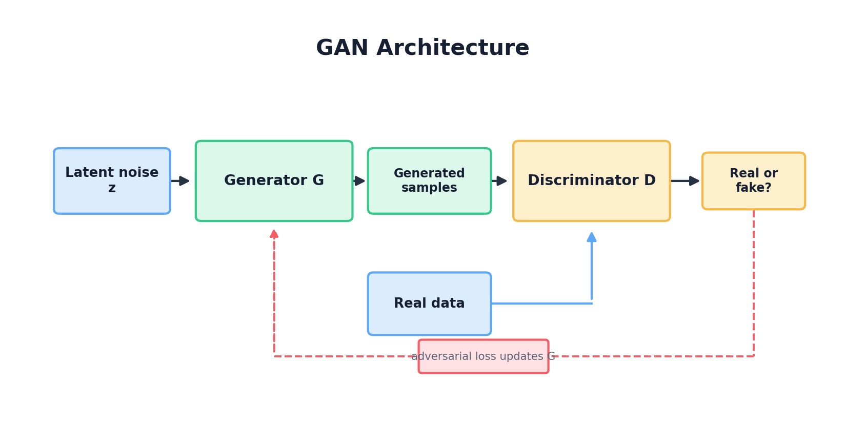
A GAN consists of two neural networks locked in competition. The generator G takes random noise and transforms it into synthetic data. The discriminator D attempts to distinguish real data from fake. During training, G improves at fooling D, while D sharpens its ability to detect fakes. At equilibrium, G produces indistinguishable samples and D achieves 50% accuracy (random guessing).
Mathematically, they optimize the minimax objective:
min_G max_D V(G, D) = E_x[log D(x)] + E_z[log(1 - D(G(z)))]Where x is real data, z is random noise, D(x) outputs the probability that x is real, and the two terms reflect the discriminator's dual goal: maximize the log-likelihood of correctly classifying real samples (first term) and fake samples (second term).
Training Dynamics and Mode Collapse
The theoretical elegance of this formulation belies practical challenges. In early training, D easily distinguishes real from fake. The gradient ∇_z log(1 − D(G(z))) becomes very small for poor samples, causing G's updates to stall. This is why practitioners use the non-saturating objective max_G log D(G(z)) (equivalently, minimize −log D(G(z))), which provides strong gradients even when the generator is losing badly.
More insidiously, G may discover a small set of samples that fool D, then collapse toward that mode, ignoring the rest of the data distribution. If the real data is bimodal or multimodal, the generator produces only from one cluster. Diagnosing mode collapse requires monitoring the diversity of generated samples—a challenge that occupied GAN researchers for years.
Wasserstein GANs (WGAN)
In 2017, Arjovsky et al. proposed a breakthrough: replace the Jensen-Shannon divergence (implicit in the original GAN objective) with the Wasserstein distance, or "earth mover's distance." This metric measures how much "earth" you must move to transform one distribution into another, and it remains informative even when distributions are disjoint—unlike JS divergence, which plateaus.
The WGAN objective becomes:
min_G max_D { E_x[D(x)] - E_z[D(G(z))] }Where D is 1-Lipschitz (its gradients are bounded). The original WGAN enforced this with weight clipping; the widely used WGAN-GP variant replaces clipping with a gradient penalty, which is usually more stable in practice. The payoff: more stable convergence, meaningful loss values that correlate with sample quality, and reduced mode collapse. WGAN-style objectives became a practical standard in many applications.
PyTorch Implementation: A Simple 2D GAN
Let's implement a minimal WGAN to generate data from a 2D Gaussian mixture. This example illustrates the core mechanics and common pitfalls:
import torch
import torch.nn as nn
import torch.optim as optim
import numpy as np
from torch.utils.data import DataLoader, TensorDataset

# Synthetic data: mixture of two Gaussians
def create_2d_data(n_samples=5000):
    cluster1 = np.random.randn(n_samples // 2, 2) + np.array([2, 2])
    cluster2 = np.random.randn(n_samples // 2, 2) + np.array([-2, -2])
    data = np.vstack([cluster1, cluster2]).astype(np.float32)
    return torch.FloatTensor(data)

# Generator: maps z (latent) to data space
class Generator(nn.Module):
    def __init__(self, latent_dim=2):
        super().__init__()
        self.net = nn.Sequential(
            nn.Linear(latent_dim, 128),
            nn.ReLU(),
            nn.Linear(128, 128),
            nn.ReLU(),
            nn.Linear(128, 2)
        )
        self.latent_dim = latent_dim

    def forward(self, z):
        return self.net(z)

# Discriminator: maps data to scalar (1-Lipschitz critic)
class Discriminator(nn.Module):
    def __init__(self):
        super().__init__()
        self.net = nn.Sequential(
            nn.Linear(2, 128),
            nn.LeakyReLU(0.2),
            nn.Linear(128, 128),
            nn.LeakyReLU(0.2),
            nn.Linear(128, 1)  # No sigmoid for WGAN
        )

    def forward(self, x):
        return self.net(x)

# Gradient penalty for Lipschitz constraint
def gradient_penalty(discriminator, real_data, fake_data, device, lambda_gp=10):
    batch_size = real_data.size(0)
    alpha = torch.rand(batch_size, 1, device=device)

    interpolates = (alpha * real_data + (1 - alpha) * fake_data).requires_grad_(True)
    d_interpolates = discriminator(interpolates)

    fake = torch.ones(batch_size, 1, device=device, requires_grad=True)
    gradients = torch.autograd.grad(
        outputs=d_interpolates,
        inputs=interpolates,
        grad_outputs=fake,
        create_graph=True,
        retain_graph=True,
    )[0]

    gradients = gradients.view(batch_size, -1)
    gradient_penalty = ((gradients.norm(2, dim=1) - 1) ** 2).mean() * lambda_gp
    return gradient_penalty

# Training loop
def train_wgan(epochs=50, batch_size=64, latent_dim=2, device='cpu'):
    data = create_2d_data()
    dataloader = DataLoader(TensorDataset(data), batch_size=batch_size, shuffle=True)

    G = Generator(latent_dim).to(device)
    D = Discriminator().to(device)

    opt_G = optim.Adam(G.parameters(), lr=1e-4, betas=(0.5, 0.9))
    opt_D = optim.Adam(D.parameters(), lr=1e-4, betas=(0.5, 0.9))

    for epoch in range(epochs):
        for real_data, in dataloader:
            real_data = real_data.to(device)
            batch_size = real_data.size(0)

            # Train discriminator (critic)
            for _ in range(5):  # More D updates per G update
                z = torch.randn(batch_size, latent_dim, device=device)
                fake_data = G(z).detach()

                d_real = D(real_data).mean()
                d_fake = D(fake_data).mean()
                gp = gradient_penalty(D, real_data, fake_data, device)

                d_loss = -d_real + d_fake + gp

                opt_D.zero_grad()
                d_loss.backward()
                opt_D.step()

            # Train generator
            z = torch.randn(batch_size, latent_dim, device=device)
            fake_data = G(z)
            d_fake = D(fake_data).mean()
            g_loss = -d_fake  # Maximize D(G(z))

            opt_G.zero_grad()
            g_loss.backward()
            opt_G.step()

        if (epoch + 1) % 10 == 0:
            print(f"Epoch {epoch+1}/{epochs} | D loss: {d_loss.item():.4f} | G loss: {g_loss.item():.4f}")

    return G, D

# Generate samples
device = torch.device('cuda' if torch.cuda.is_available() else 'cpu')
G, D = train_wgan(epochs=100, device=device)

z_test = torch.randn(1000, 2, device=device)
synthetic_samples = G(z_test).detach().cpu().numpy()
print(f"Generated {synthetic_samples.shape[0]} samples with shape {synthetic_samples.shape[1]}")
This code trains a WGAN to learn the bimodal Gaussian distribution. Key details:
- Gradient penalty: Enforces the 1-Lipschitz constraint without weight clipping, which was unstable.
- Multiple discriminator updates: Training D more often than G helps stabilize convergence.
- No sigmoid in discriminator: WGAN discriminators are unbounded critics, not classifiers.
- Adam hyperparameters: β₁ = 0.5 is standard for GANs; it reduces momentum and helps training converge.
3. Variational Autoencoders (VAEs)
The Encoder-Decoder Framework
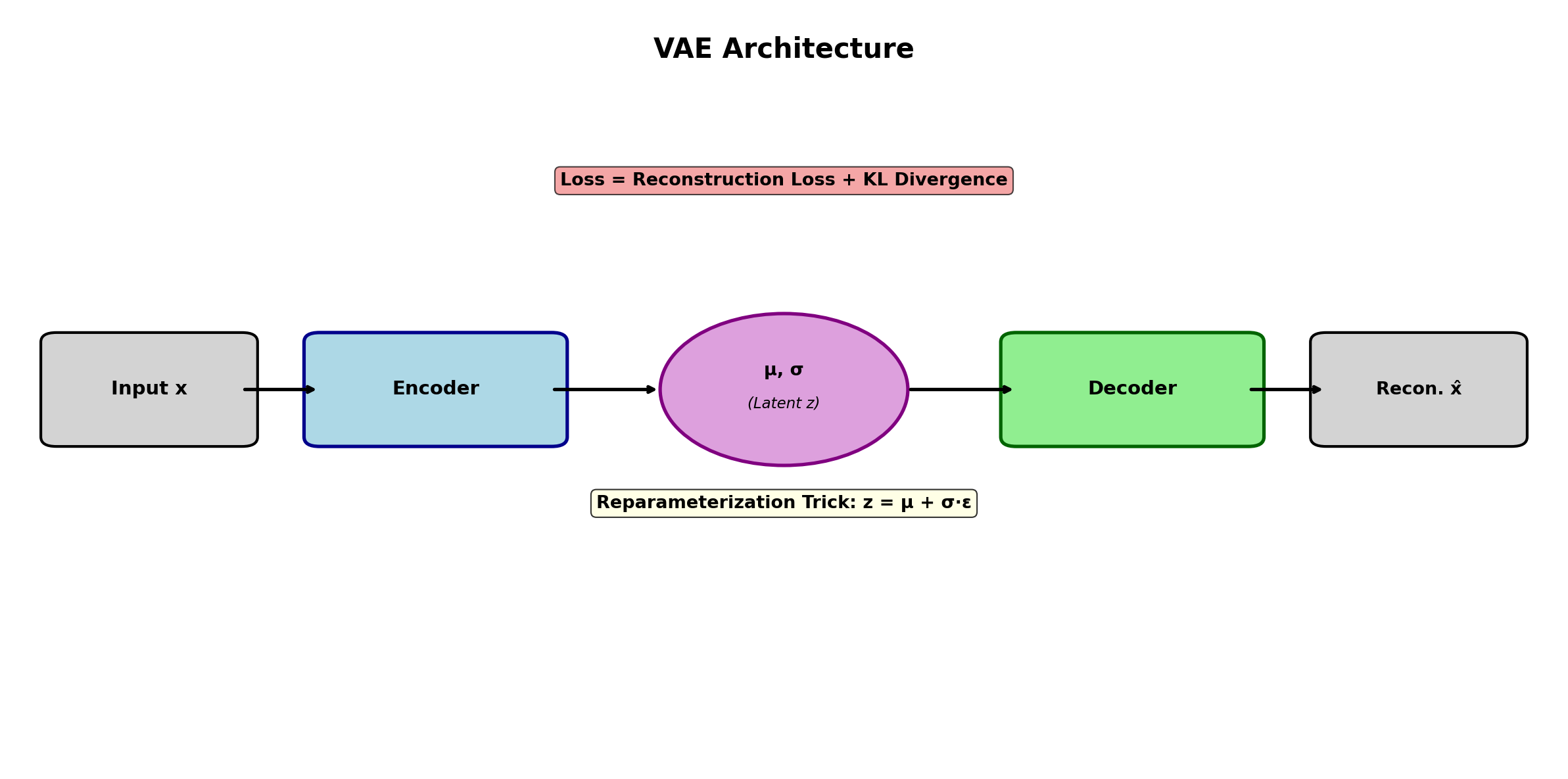
Unlike GANs, which work with noise directly, VAEs learn to compress data into a latent space and reconstruct it. An encoder maps data x to a latent representation z; a decoder reconstructs x̂ from z. But VAEs do something crucial: they learn distributions over latent codes, not point estimates. The encoder outputs mean and log-variance, defining a Gaussian posterior q(z|x).
This probabilistic view connects VAEs to the broader framework of variational inference. We seek to maximize the evidence lower bound (ELBO):
ELBO = E_q(z|x)[log p(x|z)] - KL(q(z|x) || p(z))The first term is reconstruction loss (how well the decoder recovers the original), and the second is a regularizer pushing the posterior toward a prior (usually standard normal). The tension between these terms is central to VAE behavior: strong reconstruction favors mode collapse around training data; strong regularization pushes latent space to follow a simple prior, enabling smooth interpolation and generation.
The Reparameterization Trick
To backpropagate through stochastic sampling, Kingma and Welling introduced the reparameterization trick. Instead of sampling z ~ q(z|x) directly (which breaks the gradient flow), we sample noise ε ~ N(0, I) and compute z = μ + σ ⊙ ε, where μ and log σ are encoder outputs. This makes z a deterministic function of inputs and noise, preserving gradients through the encoder.
VAE Advantages and Trade-offs
VAEs offer stability compared to GANs: the ELBO loss is tractable, training is straightforward, and mode coverage is built-in (the prior prevents collapse). They excel at learning meaningful latent spaces—interpolation between encoded samples is smooth and interpretable. However, they often produce blurrier outputs than GANs, especially for images, because the reconstruction loss encourages averaging over uncertainty.
PyTorch Implementation: A Simple VAE
import torch
import torch.nn as nn
import torch.optim as optim
from torch.utils.data import DataLoader, TensorDataset

class VAE(nn.Module):
    def __init__(self, input_dim=2, hidden_dim=128, latent_dim=2):
        super().__init__()
        self.latent_dim = latent_dim

        # Encoder: x -> [mu, log_var]
        self.encoder = nn.Sequential(
            nn.Linear(input_dim, hidden_dim),
            nn.ReLU(),
            nn.Linear(hidden_dim, hidden_dim),
            nn.ReLU()
        )
        self.fc_mu = nn.Linear(hidden_dim, latent_dim)
        self.fc_logvar = nn.Linear(hidden_dim, latent_dim)

        # Decoder: z -> x_recon
        self.decoder = nn.Sequential(
            nn.Linear(latent_dim, hidden_dim),
            nn.ReLU(),
            nn.Linear(hidden_dim, hidden_dim),
            nn.ReLU(),
            nn.Linear(hidden_dim, input_dim)
        )

    def encode(self, x):
        h = self.encoder(x)
        mu = self.fc_mu(h)
        logvar = self.fc_logvar(h)
        return mu, logvar

    def reparameterize(self, mu, logvar):
        std = torch.exp(0.5 * logvar)
        eps = torch.randn_like(std)
        z = mu + eps * std
        return z

    def decode(self, z):
        return self.decoder(z)

    def forward(self, x):
        mu, logvar = self.encode(x)
        z = self.reparameterize(mu, logvar)
        recon = self.decode(z)
        return recon, mu, logvar, z

def vae_loss(recon, x, mu, logvar, beta=1.0):
    # Reconstruction loss (MSE for continuous data)
    recon_loss = nn.functional.mse_loss(recon, x, reduction='mean')

    # KL divergence: KL(q(z|x) || p(z)) with p(z) = N(0, I)
    kl_loss = -0.5 * torch.mean(1 + logvar - mu.pow(2) - logvar.exp())

    # Total ELBO (we minimize -ELBO)
    return recon_loss + beta * kl_loss, recon_loss, kl_loss

def train_vae(data, epochs=50, batch_size=64, latent_dim=2, device='cpu'):
    dataloader = DataLoader(TensorDataset(data), batch_size=batch_size, shuffle=True)

    vae = VAE(input_dim=2, hidden_dim=128, latent_dim=latent_dim).to(device)
    optimizer = optim.Adam(vae.parameters(), lr=1e-3)

    # Annealing beta to balance reconstruction and KL (helps training stability)
    for epoch in range(epochs):
        beta = min(1.0, epoch / max(1, epochs // 2))  # Linearly anneal from 0 to 1

        for x, in dataloader:
            x = x.to(device)

            recon, mu, logvar, z = vae(x)
            loss, recon_loss, kl_loss = vae_loss(recon, x, mu, logvar, beta=beta)

            optimizer.zero_grad()
            loss.backward()
            torch.nn.utils.clip_grad_norm_(vae.parameters(), max_norm=1.0)
            optimizer.step()

        if (epoch + 1) % 10 == 0:
            print(f"Epoch {epoch+1}/{epochs} | Loss: {loss.item():.4f} | "
                  f"Recon: {recon_loss.item():.4f} | KL: {kl_loss.item():.4f}")

    return vae

# Training
data = create_2d_data()
device = torch.device('cuda' if torch.cuda.is_available() else 'cpu')
vae = train_vae(data, epochs=100, device=device)

# Generation: sample z from standard normal, decode
z_sample = torch.randn(1000, 2, device=device)
with torch.no_grad():
    synthetic_data = vae.decode(z_sample).cpu().numpy()
print(f"Generated {synthetic_data.shape[0]} samples")
Key VAE implementation details:
- Beta annealing: Starting with low β allows the reconstruction loss to dominate early, giving the encoder time to learn. Then β increases, enforcing the latent prior constraint. This improves both stability and final quality.
- Gradient clipping: Prevents exploding gradients, which can occur during KL term updates.
- Reparameterization: Sampling ε outside the model graph and using z = μ + σ ⊙ ε ensures backprop flows through both μ and σ.
4. Normalizing Flows
Invertible Transformations and Change of Variables
Normalizing flows take a different approach: rather than sampling from a latent space or training a generator, they transform a simple base distribution (e.g., standard normal) via a sequence of invertible functions. If each transformation is invertible and we know its Jacobian determinant, we can compute the density of the resulting distribution exactly.
Starting with z₀ ~ p₀(z₀), we apply transformations z₁ = f₁(z₀), z₂ = f₂(z₁), ..., zₖ = fₖ(zₖ₋₁). The density of the final sample follows from the change of variables formula:
log p(zₖ) = log p₀(z₀) - Σᵢ log |det(∂fᵢ/∂zᵢ₋₁)|This is exact, not approximate. We can directly optimize maximum likelihood. The constraint is that f must be invertible and its Jacobian must be tractable to compute.
RealNVP
A practical realization is RealNVP (Real-valued Non-Volume Preserving), which uses coupling layers. At each layer, we split dimensions into "frozen" and "transformed" parts. The transformation for the active dimensions is a function of the frozen dimensions, ensuring invertibility and tractable Jacobians (triangular structure):
y₁ = x₁
y₂ = x₂ ⊙ exp(s(x₁)) + t(x₁)
Where s (scale) and t (translation) are neural networks taking x₁ as input. Inversion is straightforward: recover x₁ from y₁, then compute x₂ = (y₂ - t(x₁)) ⊙ exp(-s(x₁)). Stacking layers with alternating which dimensions are frozen creates an expressive bijection.
Advantages and Limitations
Flows offer exact likelihood computation and fast, stable training. They're excellent for density estimation and importance sampling. However, they require invertible architectures, which constrains expressiveness, and stacking many layers increases computational cost. For very high-dimensional data (e.g., images), flows are less popular than GANs or diffusion models, though recent work (e.g., Glow) has scaled them effectively.
5. Diffusion Models
Forward and Reverse Diffusion
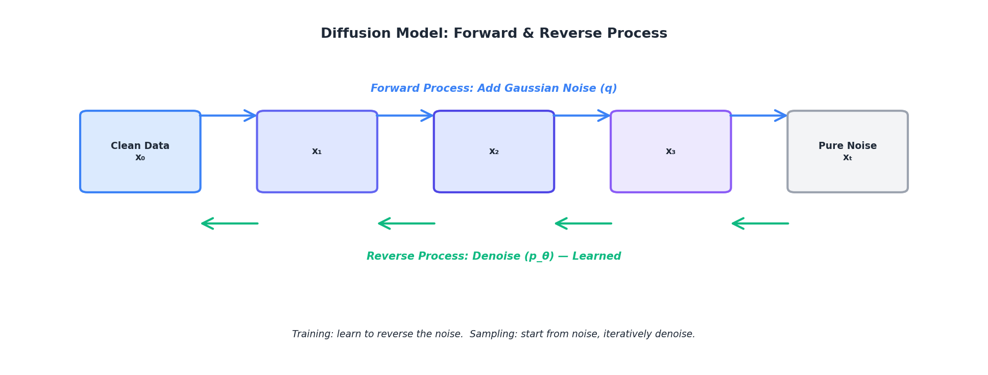
Diffusion models approach generation from a different angle: they learn to reverse a noise corruption process. The forward process gradually adds Gaussian noise to real data over T timesteps:
q(x_t | x_0) = N(x_t | √ᾱ_t x_0, (1 - ᾱ_t) I)Where ᾱ_t is the cumulative product of noise schedules and decreases monotonically from 1 down to 0 as t goes from 0 to T. At t = 0, ᾱ_t ≈ 1 and the sample is essentially clean data; at t = T, ᾱ_t ≈ 0 and the sample is pure Gaussian noise. The reverse process learns to denoise: starting from noise, iteratively remove Gaussian noise to recover data:
p(x_{t-1} | x_t) = N(x_{t-1} | μ_θ(x_t, t), σ_t² I)A neural network μ_θ (parameterized by θ) predicts the mean at each reverse step.
Training and the Score Matching Objective
Rather than directly predicting the mean, modern implementations use score matching: the network predicts the gradient of log-density, called the score. Training minimizes the expected squared difference between predicted and true scores:
L = E_t E_x₀ E_ε [ || ε_θ(x_t, t) - ε ||² ]Where ε_θ predicts the noise added in the forward process, and ε ~ N(0, I). This is simpler than direct mean prediction and has better empirical properties. The model is conditioned on timestep t, typically via sinusoidal positional embeddings (borrowed from Transformer architectures).
DDPM: Denoising Diffusion Probabilistic Models
DDPM formalized this framework, showing that diffusion models could match or exceed GAN quality on image generation. The algorithm:
- Sample x₀ from training data, noise level t ~ Uniform(1, T), and noise ε ~ N(0, I).
- Compute noisy sample x_t via forward process.
- Train network to predict ε from (x_t, t).
- Sample via reverse process: iteratively apply the learned denoiser.
Sampling is slower than GANs (requires T forward passes, often 50–1000), but the model is stable, mode-covering, and produces high-quality samples. Recent advances (DDIM, latent diffusion) speed up sampling with fewer steps or operate in compressed latent spaces.
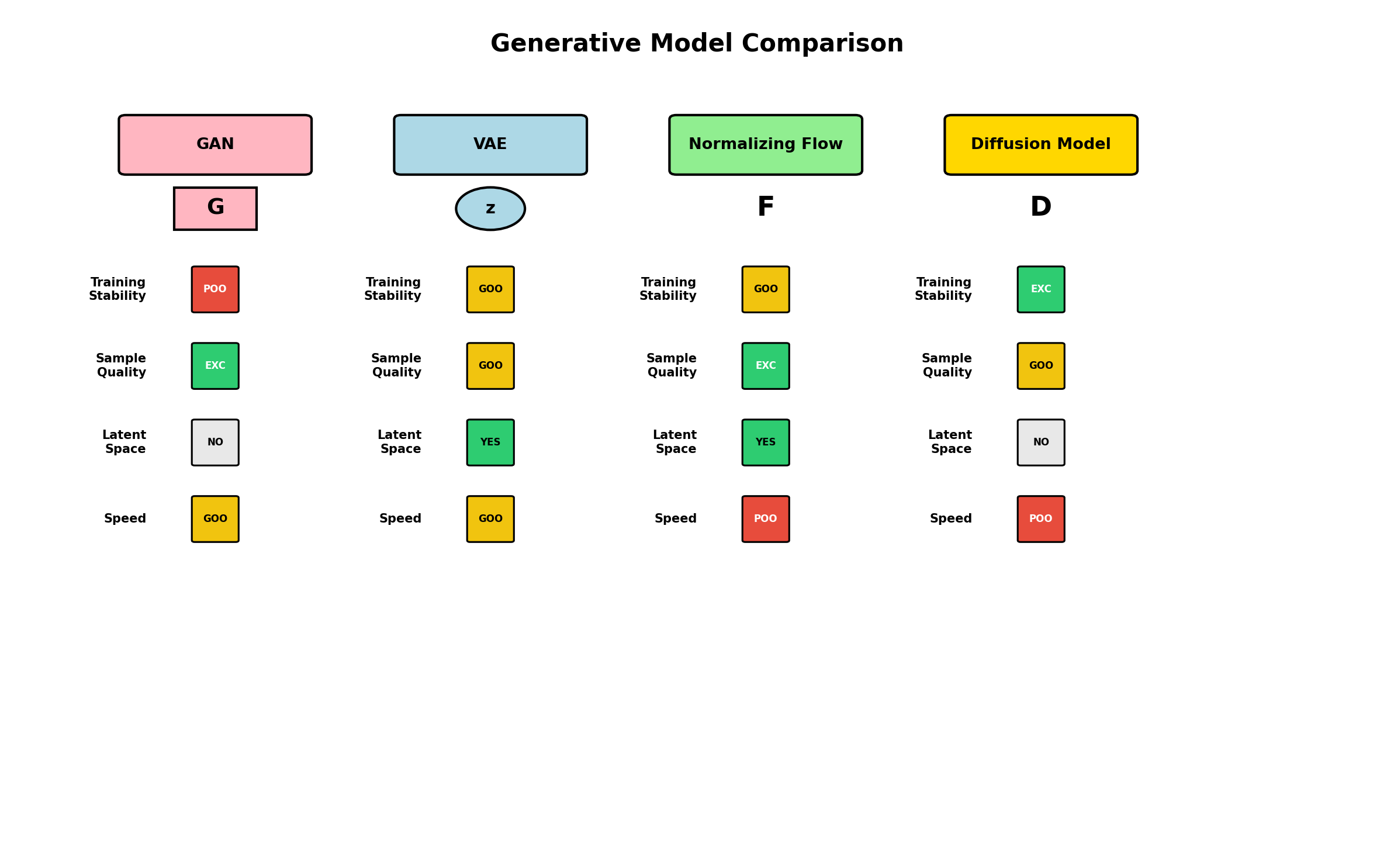
6. Comparing Approaches: When to Use Each Method
Each architecture has distinct strengths and weaknesses. The following table summarizes key trade-offs:
| Aspect | GAN | VAE | Normalizing Flow | Diffusion |
|---|---|---|---|---|
| Sample Quality | Excellent (sharp) | Good (blurry) | Very Good | Excellent |
| Sampling Speed | Very Fast | Fast | Moderate | Slow (50-1000 steps) |
| Training Stability | Unstable | Stable | Stable | Very Stable |
| Likelihood Evaluation | No (implicit) | Lower bound | Exact | Intractable |
| Mode Coverage | Often poor | Good | Good | Excellent |
| Implementation Complexity | Medium | Low-Medium | High | Medium |
| Best Use Case | Low-latency image synthesis | Representation learning, semi-supervised | Density estimation, likelihood-based tasks | High-quality synthesis, diverse outputs |
Decision Framework
Use GANs if: You need real-time synthesis (e.g., game assets, live video synthesis) and can afford dedicated engineering to stabilize training. GANs are less popular in academic settings now but remain useful for latency-critical applications.
Use VAEs if: You need both a generative model and good latent representations (e.g., for downstream classification, clustering, or semi-supervised learning). VAEs also train quickly with fewer hyperparameter surprises.
Use Normalizing Flows if: Exact likelihood evaluation is critical (e.g., density estimation, anomaly detection via log-likelihood thresholding). Flows are less commonly used for synthesis alone but excel at tasks requiring both generation and density estimation.
Use Diffusion Models if: Sample quality and mode coverage are paramount, and sampling latency is acceptable. Diffusion models are the current state-of-the-art for image synthesis and have proven effective for audio, video, and structured data.
7. Training Tips and Common Pitfalls
General Best Practices
- Monitor multiple metrics: Plot generator/discriminator loss, sample quality metrics (FID for images), and diversity measures. A single loss value hides imbalance.
- Use validation-based checkpointing: Save model snapshots based on validation metrics, not training loss. For GANs, save the generator every N iterations and later pick the one with best FID.
- Hyperparameter sensitivity: Learning rates, batch sizes, and architecture details heavily influence convergence. Start with published baselines and vary one hyperparameter at a time.
- Data preprocessing: Normalize inputs to reasonable ranges (e.g., [-1, 1] for images, standardized for tabular data). Bad preprocessing leads to training collapse.
- Batch normalization effects: Batch norm can introduce instability in GANs due to dependence on batch composition. Consider layer norm or group norm as alternatives.
- Architecture design: Use residual connections, skip connections, and attention mechanisms to improve stability and expressiveness. Modern networks often combine ideas from ResNets, Transformers, and classical deep learning.
8. From Images to Structured Data
While deep generative models were developed for images, they apply broadly to other modalities. The key is adapting the architecture and loss function to the data type.
Tabular Data
Tabular data is mixed-type (continuous, categorical, ordinal) and often sparse. GANs adapted for tabular data (e.g., TVAE, CTGAN) use tricks like:
- Gumbel-softmax for categorical sampling, differentiable but discrete.
- Per-column normalization to handle features with different scales and distributions.
- Mode-specific loss weighting to handle imbalanced classes.
VAEs for tabular data use similar techniques but naturally handle mixed types through conditional distributions in the decoder (Gaussian for continuous, categorical for discrete).
Time Series
Time series require temporal structure. Recurrent networks (LSTM, GRU) or Transformers replace fully-connected layers. A common approach:
- Encoder: LSTM that reads the entire sequence and outputs a latent vector.
- Decoder: Another LSTM that generates the sequence step-by-step from the latent vector.
- Loss: MSE on the full sequence, plus any VAE regularization (KL).
Recent diffusion models for time series (e.g., DiffWave, TimeGrad) treat time series as corrupted by noise and iteratively denoise, achieving strong results.
Graphs
Graph-structured data requires different networks. Graph neural networks (GNNs) embed nodes and edges jointly. Generative models for graphs often use:
- Autoregressive approaches: Generate one node/edge at a time, conditioning on previously generated elements.
- VAE + GNN encoder/decoder: Encoder uses GNN to embed the graph, decoder reconstructs via another GNN.
- Diffusion on graphs: Noise and denoise graph structure iteratively.
Graph generation is active research and more complex than images, but the core principles (latent representations, denoising, adversarial training) transfer directly.
9. Hands-On: Training a Simple GAN from Scratch
Let's build a complete, minimal example that generates synthetic data from a known distribution. This walkthrough covers setup, training, and evaluation.
Complete Training Script
import torch
import torch.nn as nn
import torch.optim as optim
import numpy as np
import matplotlib.pyplot as plt
from torch.utils.data import DataLoader, TensorDataset

# Step 1: Create synthetic target data
# Goal: Generator learns to produce samples from a bimodal Gaussian mixture
np.random.seed(42)
torch.manual_seed(42)

n_samples = 5000
cluster1 = np.random.randn(n_samples // 2, 2) * 0.5 + np.array([2, 0])
cluster2 = np.random.randn(n_samples // 2, 2) * 0.5 + np.array([-2, 0])
real_data = np.vstack([cluster1, cluster2]).astype(np.float32)
real_data_tensor = torch.FloatTensor(real_data)

# Step 2: Define generator and discriminator
class SimpleGenerator(nn.Module):
    def __init__(self, latent_dim=2):
        super().__init__()
        self.model = nn.Sequential(
            nn.Linear(latent_dim, 256),
            nn.ReLU(),
            nn.Linear(256, 256),
            nn.ReLU(),
            nn.Linear(256, 2)
        )

    def forward(self, z):
        return self.model(z)

class SimpleDiscriminator(nn.Module):
    def __init__(self):
        super().__init__()
        self.model = nn.Sequential(
            nn.Linear(2, 256),
            nn.LeakyReLU(0.2),
            nn.Linear(256, 256),
            nn.LeakyReLU(0.2),
            nn.Linear(256, 1)
        )

    def forward(self, x):
        return self.model(x)

# Step 3: Initialize models and optimizers
device = torch.device('cuda' if torch.cuda.is_available() else 'cpu')
generator = SimpleGenerator(latent_dim=2).to(device)
discriminator = SimpleDiscriminator().to(device)

lr = 0.0002
beta1, beta2 = 0.5, 0.999
opt_G = optim.Adam(generator.parameters(), lr=lr, betas=(beta1, beta2))
opt_D = optim.Adam(discriminator.parameters(), lr=lr, betas=(beta1, beta2))

criterion = nn.BCEWithLogitsLoss()

# Step 4: Training loop
num_epochs = 200
batch_size = 64
dataloader = DataLoader(TensorDataset(real_data_tensor), batch_size=batch_size, shuffle=True)

g_losses, d_losses = [], []

for epoch in range(num_epochs):
    for batch_idx, (real_batch,) in enumerate(dataloader):
        real_batch = real_batch.to(device)
        batch_size_actual = real_batch.size(0)

        # Labels
        real_labels = torch.ones(batch_size_actual, 1, device=device)
        fake_labels = torch.zeros(batch_size_actual, 1, device=device)

        # Train Discriminator
        # Real data
        d_real_output = discriminator(real_batch)
        d_real_loss = criterion(d_real_output, real_labels)

        # Fake data
        z = torch.randn(batch_size_actual, 2, device=device)
        fake_batch = generator(z).detach()
        d_fake_output = discriminator(fake_batch)
        d_fake_loss = criterion(d_fake_output, fake_labels)

        d_loss = d_real_loss + d_fake_loss
        opt_D.zero_grad()
        d_loss.backward()
        opt_D.step()

        # Train Generator
        z = torch.randn(batch_size_actual, 2, device=device)
        fake_batch = generator(z)
        d_fake_output = discriminator(fake_batch)

        # Generator tries to fool discriminator (fake samples should look real)
        g_loss = criterion(d_fake_output, real_labels)

        opt_G.zero_grad()
        g_loss.backward()
        opt_G.step()

    g_losses.append(g_loss.item())
    d_losses.append(d_loss.item())

    if (epoch + 1) % 50 == 0:
        print(f"Epoch [{epoch+1}/{num_epochs}] | D Loss: {d_loss.item():.4f} | G Loss: {g_loss.item():.4f}")

# Step 5: Generate and visualize samples
generator.eval()
with torch.no_grad():
    z_test = torch.randn(2000, 2, device=device)
    fake_samples = generator(z_test).cpu().numpy()

# Plot results
fig, axes = plt.subplots(1, 3, figsize=(15, 4))

# Real data
axes[0].scatter(real_data[:, 0], real_data[:, 1], alpha=0.5, s=10)
axes[0].set_title('Real Data')
axes[0].set_xlim(-4, 4)
axes[0].set_ylim(-3, 3)

# Generated data
axes[1].scatter(fake_samples[:, 0], fake_samples[:, 1], alpha=0.5, s=10, color='orange')
axes[1].set_title('Generated Data')
axes[1].set_xlim(-4, 4)
axes[1].set_ylim(-3, 3)

# Training curves
axes[2].plot(g_losses, label='Generator Loss')
axes[2].plot(d_losses, label='Discriminator Loss')
axes[2].set_xlabel('Epoch')
axes[2].set_ylabel('Loss')
axes[2].legend()
axes[2].set_title('Training Curves')

plt.tight_layout()
plt.savefig('gan_results.png', dpi=150)
plt.show()

# Step 6: Quantitative evaluation
from scipy.stats import ks_2samp

# Kolmogorov-Smirnov test for each dimension
ks_dim0 = ks_2samp(real_data[:, 0], fake_samples[:, 0])
ks_dim1 = ks_2samp(real_data[:, 1], fake_samples[:, 1])

print(f"\nKS Test (Dimension 0): statistic={ks_dim0.statistic:.4f}, p-value={ks_dim0.pvalue:.4f}")
print(f"KS Test (Dimension 1): statistic={ks_dim1.statistic:.4f}, p-value={ks_dim1.pvalue:.4f}")
print("(KS is per-dimension only; a small statistic does not prove that the "
"joint 2-D distributions match — always inspect the scatter plot too.)")Walkthrough and Key Observations
- Data Creation: We define a target distribution (bimodal Gaussian). The generator must learn this.
- Architecture: Simple MLPs suffice for 2D data. In practice, use convolutions for images or other domain-specific layers.
- Training Loop: Standard GAN training: alternate discriminator and generator updates. We use BCE loss with logits for stability.
- Visualization: Scatter plots show whether the generator captures both modes. If it collapses to one cluster, mode collapse has occurred.
- Evaluation: Kolmogorov-Smirnov test quantifies distributional similarity. For real applications, use Wasserstein distance, FID (Fréchet Inception Distance for images), or task-based metrics (downstream classifier accuracy).
Running this script should show the generator gradually learning to produce samples from both clusters. The generator loss should decrease, and the scatter plot of generated samples should eventually resemble the real data distribution.
Conclusion
Deep generative models have revolutionized synthetic data generation, moving from hand-crafted statistical models to learned, implicit representations. Each approach—GANs, VAEs, Normalizing Flows, and Diffusion Models—embodies a different philosophy and trade-off:
- GANs excel at sharp, photorealistic synthesis but require careful training.
- VAEs provide stable, interpretable latent spaces and probabilistic inference.
- Normalizing Flows offer exact likelihood evaluation for density estimation.
- Diffusion Models combine stability, quality, and mode coverage, emerging as the state-of-the-art.
No single method dominates all scenarios. Practitioners must understand the strengths and weaknesses of each, choose appropriately for their domain (images, tabular data, sequences, graphs), and invest in careful implementation and hyperparameter tuning. The code examples in this chapter provide starting points; extending them to real-world data, larger scales, and domain-specific variations is the next step on your journey.
References and Further Reading
- (2014). Generative Adversarial Nets. Advances in Neural Information Processing Systems. papers.nips.cc/paper/5423-generative-adversarial-nets
- (2014). Auto-Encoding Variational Bayes. International Conference on Learning Representations. arxiv.org/abs/1312.6114
- (2015). Variational Inference with Normalizing Flows. International Conference on Machine Learning. arxiv.org/abs/1505.05770
- (2017). Density Estimation using Real NVP. International Conference on Learning Representations. arxiv.org/abs/1605.08803
- (2017). Wasserstein GAN. International Conference on Machine Learning. arxiv.org/abs/1701.07875
- (2017). Improved Training of Wasserstein GANs. Advances in Neural Information Processing Systems. arxiv.org/abs/1704.00028
- (2015). Deep Unsupervised Learning using Nonequilibrium Thermodynamics. International Conference on Machine Learning. proceedings.mlr.press/v37/sohl-dickstein15.html
- (2020). Denoising Diffusion Probabilistic Models. Advances in Neural Information Processing Systems. arxiv.org/abs/2006.11239
- (2022). High-Resolution Image Synthesis with Latent Diffusion Models. IEEE/CVF Conference on Computer Vision and Pattern Recognition. openaccess.thecvf.com