Chapter 7 — Synthetic Images, Video & Audio

1. Visual Data: The Hardest Modality

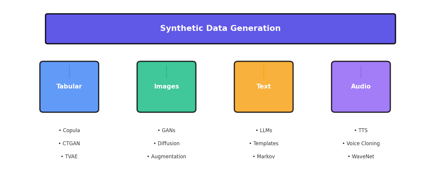
Synthetic image, video, and audio generation represents the frontier of synthetic data creation—and for good reason. Unlike tabular data where simple statistical methods often suffice, or text where pre-trained language models can perform transfer learning effectively, visual and audio modalities demand extreme computational power and extraordinary quality control.

The fundamental challenge lies in the dimensionality and perceptual sensitivity of visual data. A single 256×256 RGB image contains 196,608 values. Small errors in individual pixels that would go unnoticed in numerical data become jarring artifacts in images. A model must not only generate plausible pixels but ensure they form coherent objects with proper spatial relationships, lighting, shadows, and reflections—tasks that require understanding 3D geometry and physics that humans take for granted.

Video compounds this challenge by adding temporal consistency. Frames cannot just be individually plausible; they must flow smoothly, with objects moving predictably and physical laws respected across time. Audio adds another layer of complexity: spectrograms must align with speech articulation patterns, background noise must be realistic, and the sample rates must be high enough for human perception (typically 16 kHz or higher for speech).

2. Data Augmentation vs. Generation

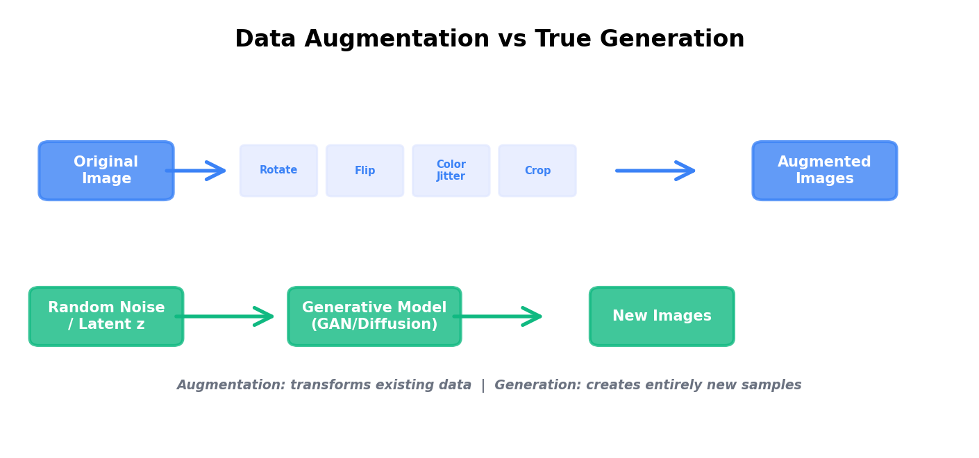
Before diving into generative models, it's critical to understand the distinction between augmentation and generation. Data augmentation modifies existing images through transformations that preserve semantic meaning: rotating, flipping, adjusting colors, cropping. It's cheap, interpretable, and often sufficient for many computer vision tasks.

True generation, by contrast, creates entirely new images from scratch or from noise. A generated image may depict a face that never existed, an object in an unseen configuration, or a scene with novel combinations of elements. Generation is far more computationally expensive but unlocks scenarios where augmentation alone fails: generating minority classes, creating adversarial examples, or simulating conditions absent from your training data.

Classic Data Augmentation with torchvision

Here's a practical augmentation pipeline using PyTorch's torchvision library:

import torch
import torchvision.transforms as transforms
from torchvision.datasets import CIFAR10
from torch.utils.data import DataLoader

# Define a comprehensive augmentation pipeline
train_transform = transforms.Compose([
    transforms.RandomHorizontalFlip(p=0.5),
    transforms.RandomVerticalFlip(p=0.1),
    transforms.RandomRotation(degrees=15),
    transforms.ColorJitter(
        brightness=0.2,
        contrast=0.2,
        saturation=0.2,
        hue=0.1
    ),
    transforms.RandomAffine(
        degrees=10,
        translate=(0.1, 0.1),
        scale=(0.9, 1.1)
    ),
    transforms.GaussianBlur(kernel_size=3, sigma=(0.1, 2.0)),
    transforms.RandomPerspective(distortion_scale=0.2, p=0.5),
    transforms.ToTensor(),
    transforms.Normalize(
        mean=[0.4914, 0.4822, 0.4465],
        std=[0.2023, 0.1994, 0.2010]
    )
])

# Test transformation pipeline
test_transform = transforms.Compose([
    transforms.ToTensor(),
    transforms.Normalize(
        mean=[0.4914, 0.4822, 0.4465],
        std=[0.2023, 0.1994, 0.2010]
    )
])

# Create dataset with augmentation
train_dataset = CIFAR10(
    root='./data',
    train=True,
    download=True,
    transform=train_transform
)

train_loader = DataLoader(
    train_dataset,
    batch_size=32,
    shuffle=True,
    num_workers=4
)

# Iterate and verify augmentation
for images, labels in train_loader:
    print(f"Batch shape: {images.shape}")
    print(f"Label shape: {labels.shape}")
    break

3. GANs for Images

Generative Adversarial Networks (GANs) were introduced by Goodfellow et al. in 2014 and revolutionized synthetic image generation. A GAN consists of two neural networks locked in competition: a generator that creates fake images and a discriminator that tries to distinguish real from fake.

The generator learns by receiving feedback from the discriminator: "your image looks too blurry" or "that face has wrong proportions." Over time, the generator improves until the discriminator can no longer tell real from fake. This adversarial dynamic has proven remarkably effective.

StyleGAN and Architecture Evolution

StyleGAN (2019) was a watershed moment in GAN research. Rather than feeding noise directly into the generator, StyleGAN uses a style mapping network that converts random latent vectors into "style codes" that control different aspects of the generated image at different scales. This separation allows fine-grained control over image properties.

Key innovations that made StyleGAN work:

• Adaptive Instance Normalization (AdaIN): Scales and shifts feature maps based on style codes, allowing style information to be injected at multiple layers.
• Progressive Training: Start generating low-resolution images (4×4) and gradually increase resolution (8×8, 16×16, ..., 1024×1024), stabilizing training and improving sample quality.
• Improved Loss Functions: Spectral normalization and other regularization techniques prevent mode collapse (where the generator produces limited varieties of images).
• Mixing Regularization: Forces different style codes to control different resolution levels, preventing the network from ignoring the latent code structure.

ProGAN (Progressive GAN) introduced the progressive training strategy, which has become standard practice. BigGAN extended this approach to class-conditional generation, allowing you to specify what class of object to generate.

4. Diffusion Models for Images

Diffusion models have recently emerged as a more stable and controllable alternative to GANs for image generation. Rather than having two networks compete, a diffusion model learns to gradually denoise random noise into coherent images.

The process has two stages:

• Forward Diffusion: Progressively add Gaussian noise to a real image until it becomes pure noise (a stochastic corruption process with a deterministic noise schedule).
• Reverse Diffusion: Learn to reverse this process—starting from noise, predict and remove noise at each step until a clean image remains.

How Stable Diffusion and DALL-E Work

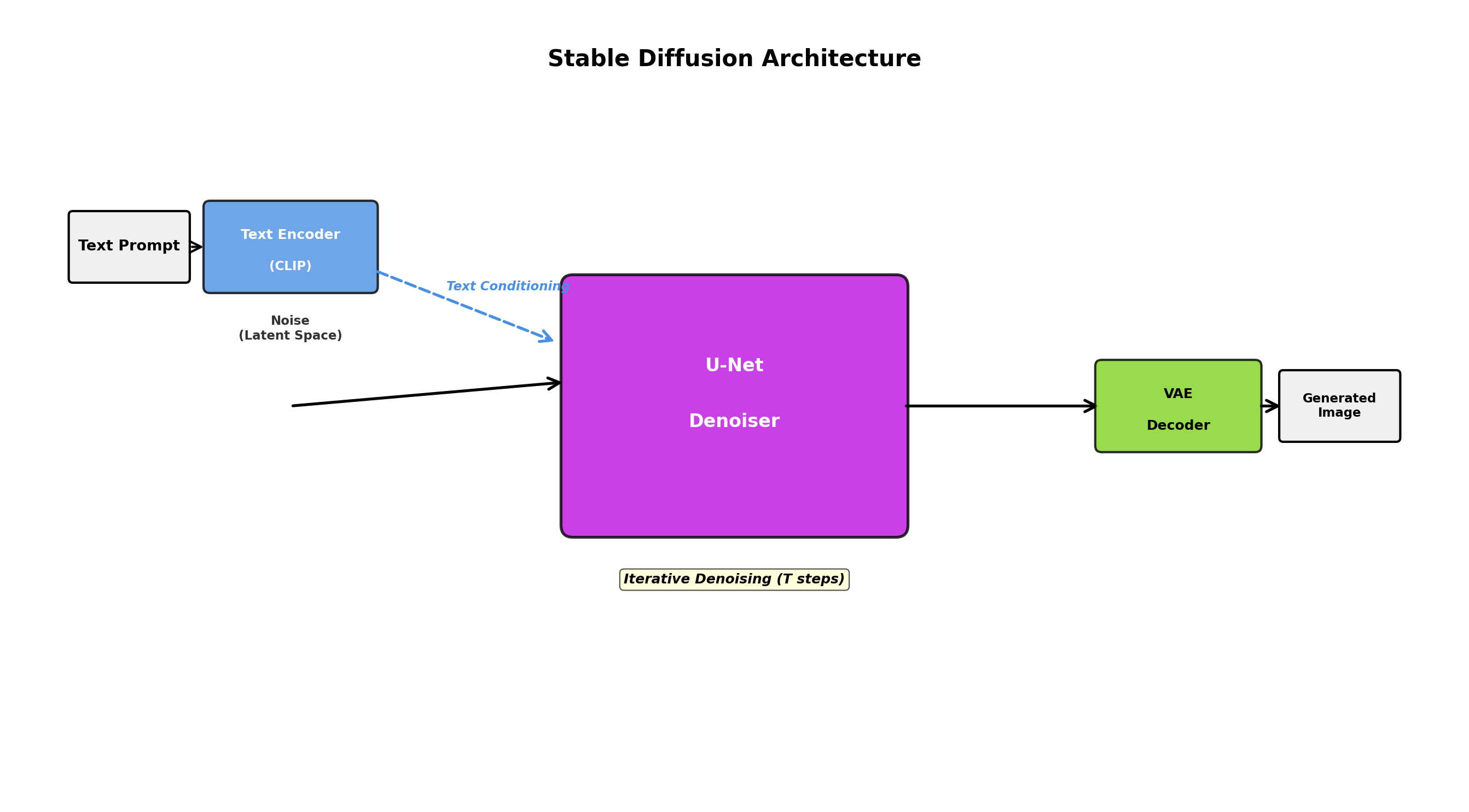
Stable Diffusion and DALL-E implement text-to-image generation by conditioning the diffusion process on text embeddings. Here's the conceptual flow:

1. Encode text prompt into embedding space using a pre-trained language model (CLIP for Stable Diffusion).
2. Initialize random noise in image space.
3. Iteratively denoise, at each step conditioning the denoising network on the text embedding.
4. After many denoising steps (typically 20-50), produce a high-quality image matching the text description.

Here's a simplified conceptual view of the denoising process:

import torch
import torch.nn as nn
from torch.nn import functional as F

class SimpleDiffusionModel(nn.Module):
    """Simplified diffusion model for educational purposes"""

    def __init__(self, image_size=32, channels=3):
        super().__init__()
        self.image_size = image_size
        self.channels = channels

        # U-Net style architecture for denoising
        self.encoder = nn.Sequential(
            nn.Conv2d(channels + 1, 64, 3, padding=1),
            nn.ReLU(),
            nn.Conv2d(64, 128, 3, padding=1),
            nn.ReLU(),
            nn.MaxPool2d(2)
        )

        self.decoder = nn.Sequential(
            nn.Upsample(scale_factor=2),
            nn.Conv2d(128, 64, 3, padding=1),
            nn.ReLU(),
            nn.Conv2d(64, channels, 3, padding=1)
        )

    def add_noise(self, x, t):
        """Add noise to image at timestep t (linear schedule)"""
        noise = torch.randn_like(x)
        alpha = 1.0 - (t / 1000.0)  # simplified schedule
        return torch.sqrt(torch.tensor(alpha)) * x + torch.sqrt(1 - alpha) * noise, noise

    def forward(self, x, t):
        """Predict noise at timestep t"""
        # Concatenate timestep information as an extra channel
        t_normalized = t.float() / 1000.0
        t_channel = t_normalized.view(-1, 1, 1, 1).expand(-1, 1, self.image_size, self.image_size)

        x_with_t = torch.cat([x, t_channel], dim=1)

        # Encode-decode architecture
        encoded = self.encoder(x_with_t)
        noise_pred = self.decoder(encoded)

        return noise_pred

    def sample(self, num_samples, device):
        """Generate images from pure noise"""
        x = torch.randn(num_samples, self.channels, self.image_size, self.image_size).to(device)

        # Iteratively denoise
        for t in range(999, 0, -1):
            with torch.no_grad():
                noise_pred = self.forward(x, torch.tensor([t] * num_samples).to(device))
                # Update x by removing predicted noise
                x = x - 0.01 * noise_pred

        return x

5. Synthetic Images for Computer Vision

One of the most practical applications of synthetic image generation is creating training data for computer vision models when real data is scarce, expensive, or contains privacy concerns.

Object Detection and Segmentation

Consider training an object detector for rare industrial defects. You have 500 real examples, but modern deep learning models need thousands. Synthetic data helps:

• Generate thousands of defects with exact bounding box annotations (no labeling cost).
• Create defects under varying lighting, camera angles, and backgrounds.
• Oversample rare defect types to balance your dataset.
• Generate edge cases (extreme lighting, partial occlusion) that might be rare in natural data.

Medical Imaging

Medical imaging is a prime use case for synthetic data due to privacy sensitivity and annotation cost. Generative models can create synthetic CT, MRI, or X-ray images that maintain realistic anatomical features while protecting patient privacy. This is particularly valuable for:

• Training segmentation models for organs or lesions.
• Balancing rare disease representations.
• Creating training data for diagnostic tasks while adhering to HIPAA and GDPR regulations.

Example: A hospital has 200 chest X-rays with pneumonia annotations but 5,000 healthy X-rays. Synthetic pneumonia cases can balance the dataset, improving model generalization.

6. Domain Randomization

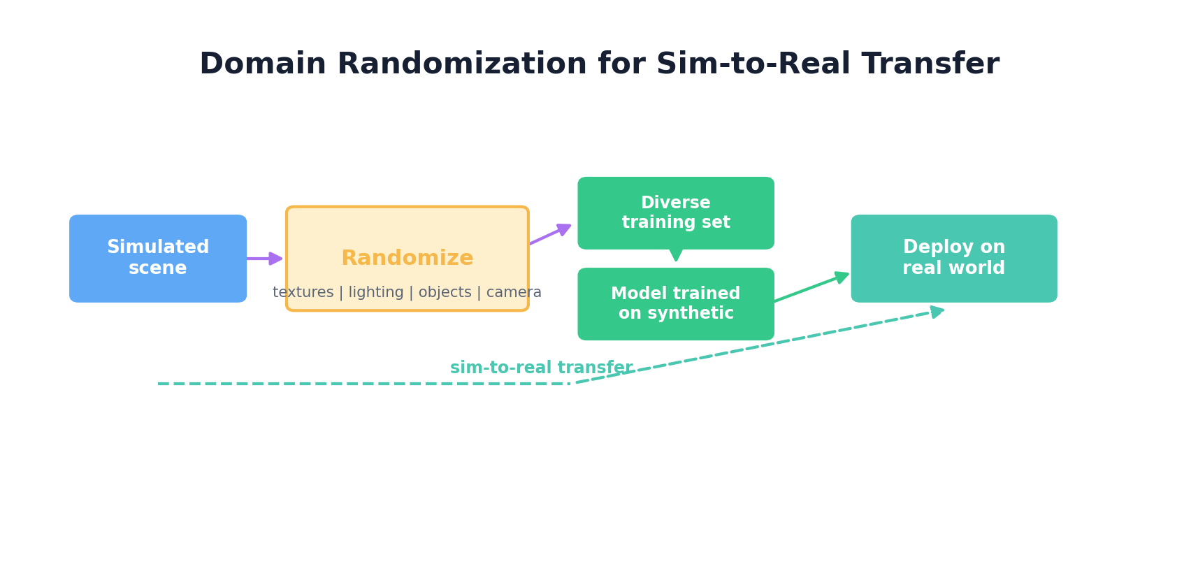
Domain randomization is a powerful technique for training models that generalize from simulation to real-world deployment. Rather than trying to make synthetic data perfectly realistic, you deliberately vary the visual properties across many random seeds, forcing the model to learn robust features that transfer across domains.

Robotics and Autonomous Vehicles

For robotics, domain randomization shines in sim-to-real transfer:

• Textures: Randomize surface textures of objects, walls, and floors at each training episode.
• Lighting: Vary light intensity, color temperature, and direction.
• Backgrounds: Sample random background images or procedurally generated scenes.
• Object Properties: Randomize size, shape, color of objects being manipulated.
• Camera Parameters: Vary focal length, resolution, and field of view.

Here's a practical example using a simulation environment:

import numpy as np
from PIL import Image, ImageDraw, ImageFilter

class DomainRandomizer:
    """Randomize visual properties for domain randomization"""

    def __init__(self, image_size=256):
        self.image_size = image_size

    def randomize_background(self, image):
        """Apply random background textures"""
        # Generate noise-based random texture
        noise = np.random.randint(0, 256, (self.image_size, self.image_size, 3), dtype=np.uint8)
        noise_img = Image.fromarray(noise)

        # Blend with original
        alpha = np.random.uniform(0.1, 0.3)
        result = Image.blend(image, noise_img, alpha)
        return result

    def randomize_lighting(self, image_array):
        """Adjust brightness and contrast randomly"""
        brightness = np.random.uniform(0.7, 1.3)
        contrast = np.random.uniform(0.7, 1.3)

        # Adjust brightness
        img = image_array.astype(np.float32)
        img = np.clip(img * brightness, 0, 255)

        # Adjust contrast (around mean)
        mean = img.mean()
        img = (img - mean) * contrast + mean
        img = np.clip(img, 0, 255)

        return img.astype(np.uint8)

    def randomize_color_jitter(self, image_array):
        """Random color channel shifts"""
        jitter = np.random.uniform(-0.2, 0.2, (1, 1, 3))
        result = np.clip(image_array.astype(np.float32) * (1 + jitter), 0, 255)
        return result.astype(np.uint8)

    def randomize_perspective(self, image):
        """Random camera angle (perspective transform)"""
        width, height = image.size
        # Random perspective coefficients
        coeffs = [
            np.random.uniform(0.9, 1.1),  # x scale
            np.random.uniform(-0.1, 0.1),  # x shear
            np.random.uniform(-10, 10),    # x translation
            np.random.uniform(-0.1, 0.1),  # y shear
            np.random.uniform(0.9, 1.1),  # y scale
            np.random.uniform(-10, 10),    # y translation
        ]
        return image.transform(
            (width, height),
            Image.PERSPECTIVE,
            coeffs,
            Image.BILINEAR
        )

    def apply_randomization(self, image):
        """Apply full domain randomization pipeline"""
        # Convert to numpy for processing
        img_array = np.array(image)

        # Random lighting
        img_array = self.randomize_lighting(img_array)
        img_array = self.randomize_color_jitter(img_array)

        # Convert back to PIL
        image = Image.fromarray(img_array)

        # Random background
        image = self.randomize_background(image)

        # Random perspective
        if np.random.rand() > 0.5:
            image = self.randomize_perspective(image)

        # Random blur
        if np.random.rand() > 0.6:
            image = image.filter(
                ImageFilter.GaussianBlur(radius=np.random.uniform(0.5, 2.0))
            )

        return image

# Usage example
randomizer = DomainRandomizer(image_size=256)
base_image = Image.open("robot_gripper.png")

# Generate multiple randomized versions for training
for i in range(10):
    randomized = randomizer.apply_randomization(base_image)
    randomized.save(f"randomized_{i}.png")

7. Synthetic Video Generation

Video synthesis introduces temporal consistency as a core challenge. Generated frames must flow smoothly, with objects moving realistically and light changing naturally across time.

Temporal Consistency and Video Diffusion

Video generation models extend image diffusion with temporal components:

• 3D Convolutions: Apply convolutions along the time dimension (not just spatial dimensions) to enforce temporal coherence.
• Optical Flow: Use optical flow estimation to ensure object motion is physically plausible.
• Frame Interpolation: Generate intermediate frames between keyframes to ensure smooth motion.
• Latent Video Diffusion: Perform diffusion in a compressed latent space (like image generation) to reduce computational cost.

OpenAI's Sora and Sora 2 illustrate how quickly the video-generation frontier moves: recent systems can generate high-quality videos from text descriptions, with stronger object consistency and temporal coherence than earlier public models. The provider landscape changes quickly, however. As of April 25, 2026, OpenAI's Help Center says the Sora web and app experiences will be discontinued on April 26, 2026, and the Sora API on September 24, 2026. Treat video-generation APIs as evolving dependencies, and verify the current roadmap before building production pipelines on any single provider.

8. Synthetic Audio & Speech

Audio synthesis has seen remarkable progress with neural vocoder and text-to-speech (TTS) systems. Unlike images where perceptual quality is heavily about pixel-level accuracy, audio quality depends on spectral properties and temporal continuity.

Text-to-Speech (TTS)

Modern TTS systems like Tacotron2, FastSpeech, and Glow-TTS work in two stages:

1. Text → Mel-spectrogram: Convert text (via phonemes) to acoustic features (mel-frequency cepstral coefficients).
2. Mel-spectrogram → Waveform: Use a neural vocoder (WaveGlow, MelGAN, HiFi-GAN) to convert acoustic features to raw audio waveforms.

Voice Cloning

Voice cloning enables generating speech in a specific person's voice with minimal samples. Techniques include:

• Speaker Embeddings: Extract voice-specific features from a short speaker sample and condition the TTS model on these embeddings.
• Style Transfer: Disentangle linguistic content from speaker characteristics, allowing synthesis of arbitrary text in a specific speaker's style.

Automatic Speech Recognition (ASR) Training Data

For low-resource languages or domain-specific ASR, synthetic speech training data helps:

• Generate speech for sentences not present in real training data.
• Augment with variations: different speakers, background noise levels, microphone qualities.
• Oversample rare phoneme combinations.

import numpy as np
from scipy import signal

class SimpleWaveformGenerator:
    """Generate synthetic speech-like audio for demonstration"""

    def __init__(self, sample_rate=16000):
        self.sample_rate = sample_rate

    def generate_tone(self, frequency, duration, amplitude=0.1):
        """Generate a pure tone at specified frequency"""
        t = np.linspace(0, duration, int(self.sample_rate * duration), False)
        waveform = amplitude * np.sin(2 * np.pi * frequency * t)
        return waveform

    def generate_speech_like_signal(self, phoneme_sequence, duration_per_phoneme=0.1):
        """Generate speech-like signal with phoneme-like formant frequencies"""
        # Simplified phoneme frequencies (formants)
        phonemes = {
            'a': [700, 1220],
            'e': [500, 2600],
            'i': [300, 2700],
            'o': [600, 1040],
            'u': [300, 870],
        }

        waveform = np.array([])
        for phoneme in phoneme_sequence:
            if phoneme in phonemes:
                formants = phonemes[phoneme]
                # Combine two formant frequencies
                tone1 = self.generate_tone(formants[0], duration_per_phoneme, amplitude=0.05)
                tone2 = self.generate_tone(formants[1], duration_per_phoneme, amplitude=0.03)
                combined = tone1 + tone2

                # Apply amplitude envelope
                envelope = signal.windows.hann(len(combined))
                combined = combined * envelope

                waveform = np.concatenate([waveform, combined])

        return waveform

    def add_background_noise(self, waveform, snr_db=20):
        """Add Gaussian noise at specified SNR"""
        noise = np.random.normal(0, 1, len(waveform))
        # Normalize noise to achieve target SNR
        signal_power = np.mean(waveform ** 2)
        noise_power = np.mean(noise ** 2)
        snr_linear = 10 ** (snr_db / 10)
        noise_scaled = noise * np.sqrt(signal_power / (snr_linear * noise_power))

        return waveform + noise_scaled

    def save_audio(self, waveform, filename, sample_rate=16000):
        """Save waveform as .wav file"""
        import wave
        # Normalize to [-1, 1]
        waveform = np.clip(waveform, -1, 1)
        # Convert to 16-bit PCM
        audio_int16 = np.int16(waveform * 32767)

        with wave.open(filename, 'w') as wav_file:
            wav_file.setnchannels(1)
            wav_file.setsampwidth(2)
            wav_file.setframerate(sample_rate)
            wav_file.writeframes(audio_int16.tobytes())

# Usage
generator = SimpleWaveformGenerator(sample_rate=16000)
phonemes = ['a', 'e', 'i', 'o', 'u']
waveform = generator.generate_speech_like_signal(phonemes, duration_per_phoneme=0.1)
waveform_with_noise = generator.add_background_noise(waveform, snr_db=15)
generator.save_audio(waveform_with_noise, 'synthetic_speech.wav')

9. 3D Synthetic Data

3D synthetic data generation uses rendering engines to create realistic scenes with precise annotations. This is critical for sensors like LiDAR and depth cameras where pixel-perfect 2D images aren't enough.

Rendering Engines: Blender and Unity

Blender (open-source) excels at:

• Procedural scene generation via Python scripting.
• Rendering high-quality images with ray tracing.
• Exporting 3D bounding boxes, depth maps, segmentation masks, and point clouds.
• Batch rendering for massive dataset generation.

Unity (game engine) is preferred for:

• Real-time rendering and simulation (robotics, autonomous driving).
• Physics simulation (object interactions, collisions).
• Photorealistic output via advanced lighting models.
• Procedural content generation via plugins.

Synthetic Data for LiDAR and Depth Sensors

Autonomous vehicles rely heavily on LiDAR (Light Detection and Ranging). Synthetic LiDAR data:

• Renders 3D scenes and computes distance to surfaces from multiple angles.
• Automatically generates point cloud annotations.
• Simulates sensor noise and occlusion.
• Scales easily (generate millions of frames vs. costly real sensor collection).

Example Blender workflow (pseudocode):

import bpy
import numpy as np
from mathutils import Vector, Euler

# Clear scene
bpy.ops.object.select_all(action='SELECT')
bpy.ops.object.delete()

# Procedurally generate scene
for i in range(20):
    # Random object placement
    bpy.ops.mesh.primitive_cube_add(
        size=np.random.uniform(0.5, 3.0),
        location=(
            np.random.uniform(-10, 10),
            np.random.uniform(-10, 10),
            np.random.uniform(0.5, 5.0)
        )
    )
    obj = bpy.context.active_object

    # Random material
    mat = bpy.data.materials.new(f"Material_{i}")
    mat.use_nodes = True
    bsdf = mat.node_tree.nodes["Principled BSDF"]
    bsdf.inputs['Base Color'].default_value = tuple(np.random.rand(3).tolist() + [1.0])

    obj.data.materials.append(mat)

# Set up camera
camera = bpy.data.objects.new("Camera", bpy.data.cameras.new("Camera"))
bpy.context.collection.objects.link(camera)
camera.location = (5, 5, 5)
camera.rotation_euler = Euler((np.radians(45), 0, np.radians(45)))
bpy.context.scene.camera = camera

# Set up lighting
light = bpy.data.objects.new("Light", bpy.data.lights.new(name="Light", type='SUN'))
bpy.context.collection.objects.link(light)
light.location = (10, 10, 10)

# Render settings
scene = bpy.context.scene
scene.render.engine = 'CYCLES'
scene.render.resolution_x = 1024
scene.render.resolution_y = 1024
scene.render.filepath = '/tmp/render.png'

# Render
bpy.ops.render.render(write_still=True)

# Export scene for annotation
bpy.ops.export_scene.obj(filepath='/tmp/scene.obj')

10. Hands-On: Augmentation Pipeline

Let's build a complete, production-ready image augmentation pipeline using torchvision and albumentations (a library offering more diverse augmentations):

import torch
import torchvision.transforms as transforms
from albumentations import (
    Compose, HorizontalFlip, VerticalFlip, Rotate,
    GaussianBlur, Perspective, CoarseDropout, Normalize
)
from albumentations.pytorch import ToTensorV2
import numpy as np
from PIL import Image
from torch.utils.data import DataLoader, Dataset

class AugmentedImageDataset(Dataset):
    """Dataset with flexible augmentation pipeline"""

    def __init__(self, image_paths, labels, augmentation=None):
        self.image_paths = image_paths
        self.labels = labels
        self.augmentation = augmentation

    def __len__(self):
        return len(self.image_paths)

    def __getitem__(self, idx):
        # Load image
        image = Image.open(self.image_paths[idx]).convert('RGB')
        image_array = np.array(image)

        # Apply augmentation
        if self.augmentation:
            augmented = self.augmentation(image=image_array)
            image_tensor = augmented['image']
        else:
            image_tensor = torch.tensor(image_array, dtype=torch.float32).permute(2, 0, 1) / 255.0

        label = self.labels[idx]
        return image_tensor, label

# Define augmentation pipelines
train_augmentation = Compose([
    HorizontalFlip(p=0.5),
    VerticalFlip(p=0.2),
    Rotate(limit=30, p=0.7),
    GaussianBlur(blur_limit=3, p=0.3),
    Perspective(scale=(0.05, 0.1), p=0.5),
    CoarseDropout(max_holes=3, max_height=16, max_width=16, p=0.3),
    Normalize(
        mean=[0.485, 0.456, 0.406],
        std=[0.229, 0.224, 0.225]
    ),
    ToTensorV2()
], bbox_params=None)

test_augmentation = Compose([
    Normalize(
        mean=[0.485, 0.456, 0.406],
        std=[0.229, 0.224, 0.225]
    ),
    ToTensorV2()
])

# Create datasets
train_dataset = AugmentedImageDataset(
    image_paths=['img1.jpg', 'img2.jpg', 'img3.jpg'],
    labels=[0, 1, 0],
    augmentation=train_augmentation
)

test_dataset = AugmentedImageDataset(
    image_paths=['test1.jpg', 'test2.jpg'],
    labels=[1, 0],
    augmentation=test_augmentation
)

# Create dataloaders
train_loader = DataLoader(train_dataset, batch_size=32, shuffle=True, num_workers=4)
test_loader = DataLoader(test_dataset, batch_size=32, shuffle=False, num_workers=4)

# Training loop snippet
model = torch.nn.Linear(224 * 224 * 3, 10)  # Placeholder
optimizer = torch.optim.Adam(model.parameters())
criterion = torch.nn.CrossEntropyLoss()

for epoch in range(5):
    for images, labels in train_loader:
        optimizer.zero_grad()
        outputs = model(images.view(images.size(0), -1))
        loss = criterion(outputs, labels)
        loss.backward()
        optimizer.step()
    print(f"Epoch {epoch+1}, Loss: {loss.item():.4f}")

Summary

Visual and audio data synthesis has matured dramatically over the past decade. From classic augmentation to GANs to diffusion models, practitioners now have multiple tools for generating synthetic data at scale. The key is matching the right technique to your constraint:

• Need variety quickly? Use augmentation pipelines.
• Need true new content? Use pre-trained diffusion models or current image-generation APIs.
• Need perfect annotations and control? Use 3D rendering engines.
• Need sim-to-real transfer? Use domain randomization.
• Need audio? Use TTS or voice cloning APIs.

The future lies in hybrid approaches: combining real and synthetic data, leveraging pre-trained models, and applying domain adaptation techniques to bridge the sim-to-real gap. As computational resources grow cheaper and these models become more accessible, synthetic visual and audio data will become the norm rather than the exception.